Excel RANK IF Formula Example

Excel has a RANK function, so you can calculate where each number stands in a list of numbers. There isn’t a RANKIF function though, if you need to rank based on criteria. Someone asked me for help with ranking daily sales, so I used COUNTIFS to make an Excel Rank If formula.

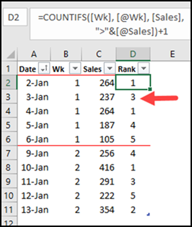
Rank Daily Sales

The goal of the Rank If formula in this example is to rank each day’s sales, compared to other days in the same week. If we just use Excel’s RANK function, it would compare each day to all the other days in the list.

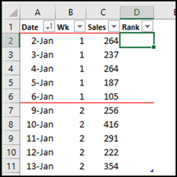
In the screen shot below, you can se the first few rows of the sample data. The sales records for two weeks are visible.

In week 1, Jan 2nd and Jan 4th have the highest sales, so they should be tied at rank of 1.
In week 2, Jan 10th has the highest sales, so it should have a rank of 1 for that week.

Get Ready to Rank the Sales

To manually rank the items largest to smallest for each week, we could count how many items are larger than each item.

In week 1, there are zero items with amounts larger than the Jan 2nd sales.
The rank for Jan 2nd is 1.
Using that information, we have a way to calculate the rank — the number of items larger, plus 1

Use COUNTIFS to Calculate RANK IF

The COUNTIFS function lets us count based on multiple criteria, so we’ll use that to create an Excel Rank IF formula.

For our criteria, we need to count:

other sales with the same week number
sales larger than the current row

Then, after COUNTIFS gives us that count, we’ll add 1 to get the rank.

To see more COUNTIFS examples, go to the the Count Functions page on my Contextures website.

The Rank IF Formula

Here’s the Rank If formula that I used for this example:

The first criterion in the formula checks for other sales with the same week number:

=COUNTIFS([Wk], [@Wk]

The second criterion find items with a larger amount in the Sales column.

Then, 1 is added to that number, to get the ranking.

Check the Ranking

To check the ranking in week 1, look at the sales for Jan 3rd — 237.

There are 2 dates with a larger sales in week 1 — Jan 2nd and Jan 4th
Add 1 to that number, and Jan 3rd has a rank of 3

Download the Sample File

To download the sample file, go to the and RANK Function page on my Contextures website. The file is in xlsx format, and does not contain macros. It contains other RANK examples too.

2 thoughts on “Excel RANK IF Formula Example”

This is so useful! And really easy to adapt to different situations.
I used this to create uneatable “Top 5” lists in a sales report.
I have a huge amount of products that are categorised under 5 segments, so instead of using the week lookup, I set my formula up to look at segment and applied the ranking to each segment.
THANKS!

Hi, i would like the above but if i have, for example, the same score in week 1 i would like the duplicate score in the same week to be the same rank number:
wk score rank
1 10 1
1 10 1
1 11 2
1 12 3

Интересно почитать: Счет в excel

Is this possible?

RANK Excel Function

By Jeevan A Y

Excel RANK Function (Table of Contents)

RANK in Excel

Rank function in excel is used for finding out the best sequence position of any selected cell from the given hierarchy or range, which is only applicable for number. And it is because Rank can only be measured in numbers. If we have 5 number and want to find the rank (or position) of any number, we simply need to select the range and then choose the order in which rank we want.

Excel functions, formula, charts, formatting creating excel dashboard & others

RANK Formula in Excel:

Below is the RANK Formula in Excel:

Explanation of RANK Function in Excel

RANK Formula in Excel includes two mandatory arguments and one optional argument.

Number: This is the value or number we want to find the rank.
Ref: This is the list of numbers in a range or in an array you want to your “Number” compared to.
[Order]: Whether you want your ranking in Ascending or Descending order. Type 0 for descending and type 1 for ascending order.

Ranking products, people, or services can help you to compare one against another. The best thing is we can see which is at the top, which is at the average level, and which is at the bottom.

We can analyze each one of them based on the rank given. If the product or service is at the bottom level, we can study that particular product or service and find the root cause for that product or service poor performance and take necessary action against them.

Three Different Types of RANK Functions in Excel

If you start typing the RANK function in excel, it will show you 3 types of RANK functions.

RANK.AVG
RANK.EQ
RANK

In Excel 2007 and earlier versions, and only the RANK Function was available. However, later on, a RANK Function has been replaced by a RANK.AVG and RANK.EQ functions.

Though RANK Function still works in recent versions, it may not be available in future versions.

How to Use RANK Function in Excel?

RANK Function in Excel is very simple and easy to use. Let understand the working of RANK Function in Excel by some RANK Formula example.

Example #1

I have a total of 12 teams that participated in the Kabaddi tournament recently. I have team names, their total points in the first two columns.

I have to rank each team when I compared it to other teams on the list.

Since RANK works only for compatibility in earlier versions, I am using RANK.EQ function instead of a RANK Function here.

Note: Both work exactly the same way.

Apply the RANK.EQ function in cell C2.

So the output will be :

We can drag the formula by using Ctrl + D or double click on the right corner of the cell C2. So the result would be:

Note: I have not mentioned the order reference. Therefore, excel by default ranks in descending order.

=RANK.EQ (B2, $B$2:$B$13) returned a number (rank) of 12. In this list, I have a total of 12 teams. This team scored 12 points, which is the lowest among all the 12 teams we have taken into consideration. Therefore, the formula ranked it as 12, i.e. the last rank.
=RANK.EQ (B3, $B$2:$B$13) returned a number (rank) of 1. This team scored 105 points, which is the highest among all the 12 teams we have taken into consideration. Therefore, the formula ranked it as 1, i.e. first rank.

Интересно почитать: Excel многопользовательский режим

This is how RANK or RANK.EQ function helps us find out each team’s rank when we compared against each other in the same group.

Example #2

One common problem with RANK.EQ function is if there are two same values, then it gives the same ranking to both the values.

Consider the below data for this example. I have a batsmen name and their career average data.

Apply the RANK.EQ function in cell C2, and the formula should like the below one.

=RANK.EQ(B2,$B$2:$B$6)

So the output will be :

We can drag the formula by using Ctrl + D or double click on the right corner of the cell C2. So the result would be:

If I apply a RANK formula to this data, both Sachin and Dravid get the rank 1.

My point is if the formula finds two duplicate values, then it has to show 1 for the first-ever value is found and the next value to the other number.

There are many ways we can find the unique ranks in these cases. In this example, I am using RANK.EQ with COUNTIF function.

So the output will be :

We can drag the formula by using Ctrl + D or double click on the right corner of the cell D2. So the result would be:

The formula I have used here is

=RANK.EQ (B2, $B$2:$B$6) this will find the rank for this set.

COUNTIF ($B$2:B2, B2) – 1. COUNTIF formula will do the magic here. For the first cell, I have mentioned $B$2:B2 means at this range, what is the total count of the B2 value then deduct that value from 1.

The first RANK returns 1 and COUNTIF returns 1, but since we mentioned -1, it becomes zero; therefore, 1+0 = 1. For Sachin, RANK remains 1.

For Dravid, we got the Rank as 2. Here RANK returns 1 but COUNTIF returns 2 but since we mentioned -1 it becomes 1 therefore 1 + 1 = 2. The rank for Dravid is 2, not 1.

This is how we can get unique ranks in case of duplicate values.

Things to Remember

A RANK Function is replaced by RANK.EQ in 2010 and later versions.
A RANK Function in Excel can accept only numerical values. Anything other than numerical values, we will get an error as #VALUE!
If the number you are testing is not present in the list of numbers, we will get #N/A! Error.
The RANK function in Excel gives the same ranking in the case of duplicate values. Anyhow, we can get unique ranks by using the COUNTIF function.
Data need not sort in ascending or descending order to get the results.

How to RANK Items in Excel Using the COUNTIFS Function

Working with data in Excel often requires you to rank data. Excel has a built-in RANK function for this purpose. But the RANK function has some limitations. One of them is RANK fails to rank data uniquely when there is duplication. You can use a neat little trick to overcome this shortcoming.

Using two COUNTIF functions together help us to rank data even if there is duplication. The COUNTIF function can also be used to rank data based on multiple criteria. In this tutorial, you will learn how to rank data using the COUNTIF function.

How to Rank in Excel rank using the COUNTIF function

You will use a high school soccer league point table data set in the next example. There are two pairs of duplicated values in this example. Using the RANK function in column C, we get the same rank for duplicated values.

To fix this issue:

Go to cell D2 and select it with your mouse.
Apply the formula to =COUNTIF($B$2:$B$8,»>»&$B2)+COUNTIF($B$2:B2,B2) cell D2.
Press Enter.
Drag the formula to the cells below.

This will rank all the values uniquely in column C with no repetitions in descending order. The first COUNTIF function is used to find out the number of values greater or less than the number that is going to be ranked. The second COUNTIF has an expanding range $B$2:B2 and extracts the number of values that are equal to the number.

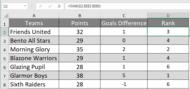
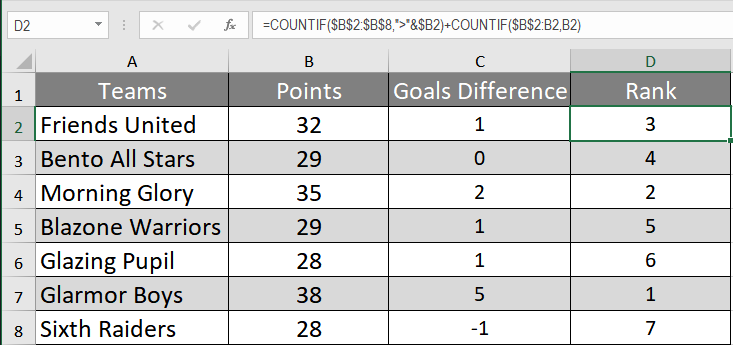
Rank in Excel Using Multiple Criteria

In the previous example, Blazone Warriors are ranked lower than Bento All Stars despite having a higher goal difference. You can use the RANK.EQ with COUNTIFS to add multiple criteria to have an improved ranking using criteria. For this example:

To fix this issue:

Go to cell D2 and select it with your mouse.
Apply the formula =RANK.EQ($B2,$B$2:$B$8)+COUNTIFS($B$2:$B$8,$B2,$C$2:$C$8,»>»&$C2) to cell D2.
Press Enter.
Drag the formula to the cells below.

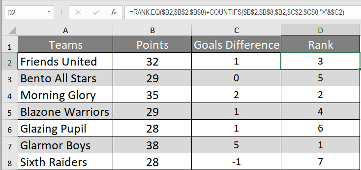
This will show Blazone Warriors ahead of Bento All Stars in the rankings. The first formula with the criteria ($B2,$B$2:$B$8) counts the number of times the values appear. The formula performs a row-wise check for the value as you have an absolute reference but a relative one for the rows ($B2).

The second formula with the criteria ($C$2:$C$8,”>”&$C2) checks how many goal differences are greater than the one being checked. This returns 0 for Blazone Warriors. However, Bento All Stars has 1 returned as the other team has a higher goal difference.

Rank in an Ascending Order using the COUNTIF function

You can rank in an ascending order using the COUNTIF function. You will use the fruit sales data in this example. To rank the sales in an ascending order:

Go to cell C2 and select it.
Apply the formula to =COUNTIF($B$2:$B$7,»<«&$B2)+COUNTIF($B$2:B2,B2) C2.
Press Enter.
Drag the formula with your mouse to the cells below.

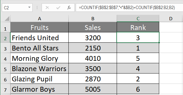
This will rank the sales in an ascending order.

Still need some help with Excel formatting or have other questions about Excel? Connect with a live Excel expert here for some 1 on 1 help. Your first session is always free.