
LOOKUP vs VLOOKUP
Knowing the difference between LOOKUP vs VLOOKUP Functions in Excel enables users to take full advantage of the benefits of using each function. The LOOKUP function LOOKUP Function The LOOKUP Function is categorized under Excel Lookup and Reference functions. The function performs a rough match lookup either in a one-row or one-column range and returns the corresponding value from another one-row or one-column range. allows a user to search for a piece of data in a row or column and return a corresponding piece of data in another row or column. The VLOOKUP function VLOOKUP Learn VLOOKUP the easy way with screenshots, examples, detailed break down of exactly how the formula works in Excel. Function =VLOOKUP(lookup value, table range, column number). For example, “look for this piece of information, in the following area, and give me some corresponding data in another column”. is similar but only allows a user to search vertically in a row and only returns data in a left-to-right procedure. This guide will outline why it’s better to use LOOKUP instead of VLOOKUP or HLOOKUP HLOOKUP Function HLOOKUP stands for Horizontal Lookup and can be used to retrieve information from a table by searching a row for the matching data and outputting from the corresponding column. While VLOOKUP searches for the value in a column, HLOOKUP searches for the value in a row. in Excel modeling.
Why use LOOKUP vs VLOOKUP or HLOOKUP?
Simply put, the LOOKUP Function is better than VLOOKUP, as it’s less restrictive in its use. It was only introduced by Microsoft in 2016, so it’s still new to most users.
Benefits of LOOKUP vs VLOOKUP:
- Users can search for data both vertically (columns) and horizontally (rows)
- Allows for left-to-right and right-to-left procedures (VLOOKUP is only left-to-right)
- Simpler to use and doesn’t require selecting the entire table
- Can replace both VLOOKUP and HLOOKUP functions
- Easier to audit with F2 than VLOOKUP or HLOOKUP
Examples of LOOKUP vs VLOOKUP
Below are two screenshots of the LOOKUP vs VLOOKUP functions being used in Excel. As you will see in both examples, there is a simple table with some people’s names, countries, and ages. The tool that’s been built allows the user to enter a person’s name and get Excel to return their age.
Example 1: LOOKUP
In this example, the LOOKUP Function is used with the following steps:
- Select the name that’s entered in cell C9.
- Search for it in column B4:B7.
- Return the corresponding age in column D4:D7.
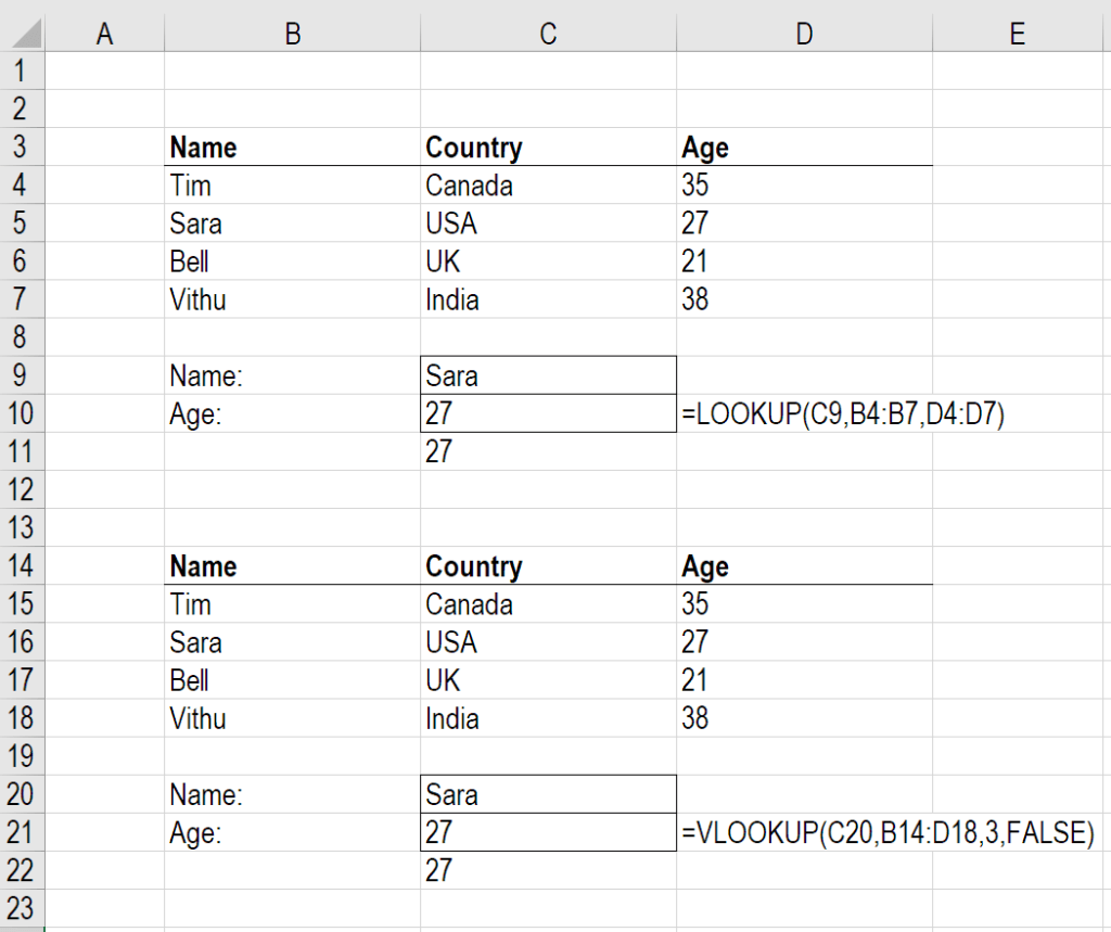
As you can see, this formula is very intuitive and easy to audit.
Example 2: VLOOKUP
In this second example, VLOOKUP is used with the following steps:
- Select the name that’s entered in cell C20.
- Select the range of the entire table B14:D18.
- Select the corresponding output from column “3.”
- “False” requires an exact name match.
This formula also works, but it’s harder to set up, understand, and audit.
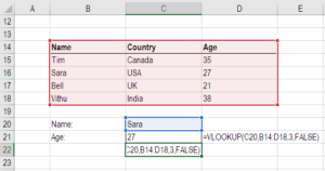
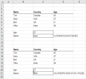
Right-to-left Functionality
The biggest benefit of LOOKUP vs VLOOKUP may be its ability to operate from right-to-left. You will see below that if you want to switch the procedure to search for age and output the corresponding name, it works for LOOKUP but produces an error with VLOOKUP.
Index Match Match Alternative
The only limitation of the LOOKUP Function is that it’s not completely dynamic. If, for example, you wanted to be able to change the output column from Age to Country, you’d need to manually change the formula to refer to a different column.
As a more advanced alternative, you can combine the INDEX and MATCH Functions to automatically switch references.
See CFI’s step by step guide on how to use Index Match Match in Excel Index Match Formula Combining INDEX and MATCH functions is a more powerful lookup formula than VLOOKUP. Learn how to use INDEX MATCH in this Excel tutorial. .
Additional Resources
Thank you for reading CFI’s explanation of the LOOKUP vs VLOOKUP functions. CFI is the official issuer of the Financial Modeling & Valuation Analyst certification program Become a Certified Financial Modeling & Valuation Analyst (FMVA)® CFI’s Financial Modeling and Valuation Analyst (FMVA)® certification will help you gain the confidence you need in your finance career. Enroll today! . To continue learning and developing as an analyst, the following free CFI resources will be helpful:
- List of Excel Functions Functions List of the most important Excel functions for financial analysts. This cheat sheet covers 100s of functions that are critical to know as an Excel analyst
- Valuation Methods Valuation Methods When valuing a company as a going concern there are three main valuation methods used: DCF analysis, comparable companies, and precedent transactions
- Excel Modeling Best Practices Excel Modeling Best Practices The following excel modeling best practices allow the user to provide the cleanest and most user-friendly modeling experience. Microsoft Excel is an extremely robust tool. Learning to become an Excel power user is almost mandatory for those in the fields of investment banking, corporate finance, and private equity.
Free Excel Tutorial
To master the art of Excel, check out CFI’s FREE Excel Crash Course, which teaches you how to become an Excel power user. Learn the most important formulas, functions, and shortcuts to become confident in your financial analysis.
How to use a VLOOKUP function in Excel VBA
VLOOKUP is one of the most useful and versatile functions in Excel. As you work further with macros it’s not uncommon to make your create an Excel VBA VLOOKUP macro. With this you get the ability to reference your tables of data, but automated.
Wait, what’s a VLOOKUP function?
The Vertical Lookup is one of Excel’s most popular commands. It’s most common use allows you retrieve data from another table of data based on a key value. For example, in one Excel sheet you may have a list of one customer’s invoice numbers, and in another sheet a list of all your invoice numbers plus other columns, such as amount, customer and invoice date. A VLOOKUP function can use the invoice number as a reference point to extract one or more other related columns of data. This avoids sloppy copy-and-paste and ensures the data remains up to date.

There are other smart uses of the VLOOKUP, such as being able to search for duplicates, group values into buckets and check to see if items exists but this is enough detail for now.
For a more thorough discussion of the VLOOKUP function, check out our article here. Even better, come on one of our Excel Advanced courses!
So what about using Excel VBA VLOOKUPs?
You can retrieve data from sheet to sheet programmatically using VBA alone, usually with nested FOR NEXT loops and variables to track your current cell position. These can be a bit fiddly and the learning curve can be a little steep (if you want to learn how to do this check out our Excel VBA Introduction / Intermediate course).

Luckily, VBA provides you with the Application.WorksheetFunction method which allows you to implement any Excel function from within your macro code.
So if your original VLOOKUP in cell B2 was something like this:
The VBA version would look like this:
Notice a couple of things: I had to insert the Sheets and Range objects so VBA could properly interpret it.
I want a sneakier version!
Don’t want to do that Sheets and Ranges business? You can adopt a little-known punctuation trick in VBA that converts things into cell references: the square brackets. Did you know you can turn this:
With a little lateral thinking we can do the same to our VLOOKUP:
Make it more robust
The code lines above will do the bare minimum. They’ll get the job done. What if you grab the result of the VLOOKUP and store it in a variable?
And then throw an unexpected value at it?

Let’s add a little error-handling so your code doesn’t come to a screeching halt. There’s a number of ways you can test this, and various things you can do with the error, so here’s only one suggestion:
The first example throws the error right up in your face. The second one is a ‘silent’ error that pushes a null string into the result variable. Not usually advisable as you can’t actually spot the problem but on some occasions you just want to move past the code issue. You could replace the empty string with your own custom error message.
Make it dynamic
This is all well and good but what if your data grows and shrinks? You should be on the lookout for dynamic methods. You can consider things such as dynamic range names and similar, but here’s a VBA option you can consider:
Note I went back to standard sheet and range references; they’re tricky to mix and match with square bracket notation.
What’s happening here? We set up three variables, to house the sheet name, last row and final range. Then we calculate what the last used row is with the “xlUp” method. This is equivalent to pressing CTRL + up on the keyboard when working in Excel. This finds the last row on the worksheet, and finally we set this as the range used.
There’s lots of variations on this, depending on whether you need dynamic columns too and how regular your data is, but this is a great method for getting you started.
So there it is, from soup to nuts, ways to implement VLOOKUP functions in Excel VBA.
Looking for help on your VBA projects? We offer the UK’s largest schedule of VBA training events, with all versions and levels trained. The Introduction and Intermediate levels will give you all the tools you need to get started, while the Advanced course will allow you to hook up other Office applications and communicate with databases. We can also visit your offices to deliver training, or consult on your projects. We can also offer Access VBA and Word VBA too.
How to Perform VLOOKUP in Power Query in Excel
VLOOKUP is one of the most popular Excel functions and there’s no doubt about it. You know this from the very beginning of your Excel journey. But today I have a something new for you, an you need to learn this right now.
Here’s the deal:
You can use POWER QUERY to match two column and get values (By using Merge Option). Yes, you heard it right, you can do VLOOKUP in Power Query.
As you know: “VLOOKUP matches values from a column and then return the values from the same row of the different column or from the same column.”
Let’s Start with Data
If you look at the below data (CLICK HERE TO DOWNLOAD) where we have two different tables with product price and category.

The one thing which is common in these two tables is product IDs. And here I want to have categories in the quantity table.
Why Power Query Instead of VLOOKUP?
As you can see we have product IDs as a common thing in both of the tables.
If you want to use VLOOKUP you need to shift product ID column before the category column in TABLE 2.
Otherwise, you can use INDEX MATCH. But here we are going to do this with Power Query.
Steps to Perform VLOOKUP with Power Query
Using Power Query to replace VLOOKUP is not just easy but fast and the best part is it’s a one-time setup.
It goes something like this:
- Create queries (connections) for the both of the tables.
- Choose the column which is common in both of the tables.
- Merge them and get the column you want.
But let’s do it step by step and make sure to download this sample file from here to follow along.
- First of all, convert both of the tables (TABLE 1 and TABLE 2) into Excel tables by using Control + T or Insert ➜ Tables ➜ Table.
- Next, you need to load data into power query editor, and for this, go to Data Tab ➜ Get & Transform Data ➜ From Table.
- After that, close the query from Home tab ➜ Close and load to ➜ Connection only. (Repeat Step 2 and 3 for the second table).

- Now from the here, right-click on the query and click “Merge” or if you are using Office 365 like me, it’s there on the Data Tab ➜ Get Data ➜ Combine Queries ➜ Merge.

- Once you click on “Merge”, it shows you the merge window.

- From this window, select the «Quantity Table» in the upper section and in the «Category Table» in down section.
- After that, select the column which is common in both of the tables (here product ID is common).

- At this point, you have a new table in the power query editor.
- From here, click on the filter button of the last column of the table and only select category (un-select Product ID) and click OK.

- Here you have a new table with category column.

- In the end, click “Close & Load” to load table into the worksheet.
BOOM! now you have a new table with category column.
Conclusion
In power query, all you have do is to create the connection for tables and merge the queries.
And the best part is, once you add new data to the quantity list new table will get updated instantly.
I hope you have found this power query tip useful, but now, tell me one thing.
Which looks better to you? Power Query or VLOOKUP?
Please share your views with me in the comment section. I’d love to hear from you, and please, don’t forget to share this post with your friends, I am sure they will appreciate it and if you want to know how to use power query in general, make sure check out this Excel Power Query Tutorial.
You must Read these Next
-
: Using power query for unpivoting a data table is a real fun. You will be surprised. : One of the best Excel options which I have learned about managing data. : Excel doesn’t allow you to refer to different worksheets. But sometimes, it happens. : In VLOOKUP, col_index_no is a static value which is the reason VLOOKUP doesn’t work like a. : Performing a two-way lookup is all about getting a value from a two-dimensional table. That means. : In this combination, both of the functions work in a sequence. VLOOKUP works in the. : A normal VLOOKUP doesn’t allow you to lookup for a value like this, but when you.
About the Author

Puneet is using Excel since his college days. He helped thousands of people to understand the power of the spreadsheets and learn Microsoft Excel. You can find him online, tweeting about Excel, on a running track, or sometimes hiking up a mountain.
Excel Tips —
 search menu
Excel Tips: How to Use Excel’s VLOOKUP Function
Lesson 19: How to Use Excel's VLOOKUP Function
How to use Excel's VLOOKUP function
Many of our learners have told us they want to learn how to use Excel's VLOOKUP function. VLOOKUP is an extremely useful tool, and learning how to use it is easier than you think!
Before you start, you should understand the basics of functions. Check out our Functions lesson from our Excel Formulas tutorial (or select a specific version of Excel). VLOOKUP works the same in all versions of Excel, and it even works in other spreadsheet applications like Гугл Sheets. You can download the example if you'd like to work along with this article.
What exactly is VLOOKUP?
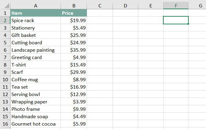
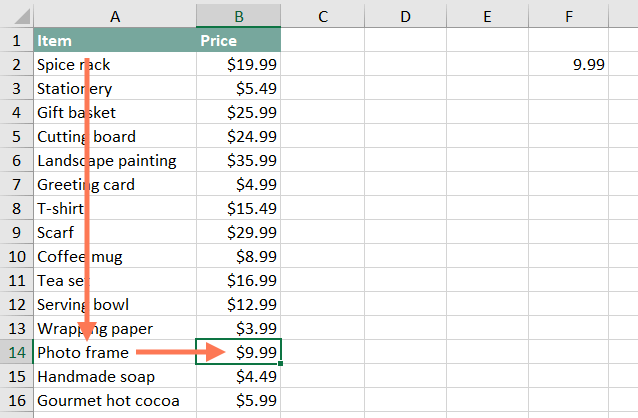
Basically, VLOOKUP lets you search for specific information in your spreadsheet. For example, if you have a list of products with prices, you could search for the price of a specific item.
We're going to use VLOOKUP to find the price of the Photo frame. You can probably already see that the price is $9.99, but that's because this is a simple example. Once you learn how to use VLOOKUP, you'll be able to use it with larger, more complex spreadsheets, and that's when it will become truly useful.
We'll add our formula to cell F2, but you can add it to any blank cell. As with any formula, you'll start with an equals sign (=). Then type the formula name. Our arguments will need to be in parentheses, so type an open parenthesis. So far, it should look like this:
=VLOOKUP(
Adding the arguments
Now, we'll add our arguments. The arguments will tell VLOOKUP what to search for and where to search.
The first argument is the name of the item you're searching for, which in this case is Photo frame. Because the argument is text, we'll need to put it in double quotes:
=VLOOKUP("Photo frame"
The second argument is the cell range that contains the data. In this example, our data is in A2:B16. As with any function, you'll need to use a comma to separate each argument:
=VLOOKUP("Photo frame", A2:B16
It's important to know that VLOOKUP will always search the first column in this range. In this example, it will search column A for "Photo frame". The value that it returns (in this case, the price) will always need to be to the right of that column.
The third argument is the column index number. It's simpler than it sounds: The first column in the range is 1, the second column is 2, etc. In this case, we are trying to find the price of the item, and the prices are contained in the second column. This means our third argument will be 2:
=VLOOKUP("Photo frame", A2:B16, 2
The fourth argument tells VLOOKUP whether to look for approximate matches, and it can be either TRUE or FALSE. If it is TRUE, it will look for approximate matches. Generally, this is only useful if the first column has numerical values that have been sorted. Because we're only looking for exact matches, the fourth argument should be FALSE. This is our last argument, so go ahead and close the parentheses:
=VLOOKUP("Photo frame", A2:B16, 2, FALSE)
That's it! When you press Enter, it should give you the answer, which is 9.99.
How it works
Let's take a look at how this formula works. It first searches vertically down the first column (VLOOKUP is short for vertical lookup). When it finds "Photo frame", it moves to the second column to find the price.
As we mentioned earlier, the price needs to be to the right of the item name. VLOOKUP cannot look to the left of the column that it's searching.
If we want to find the price of a different item, we can just change the first argument:
=VLOOKUP("T-shirt", A2:B16, 2, FALSE)
=VLOOKUP("Gift basket", A2:B16, 2, FALSE)
It would be very tedious to edit your VLOOKUP formula whenever you want to find the price of a different item. In the next example, we'll show how to avoid this by using a cell reference.
Another example
Are you ready for a slightly more advanced example? We're going to make a couple of changes to the spreadsheet to make it more realistic.
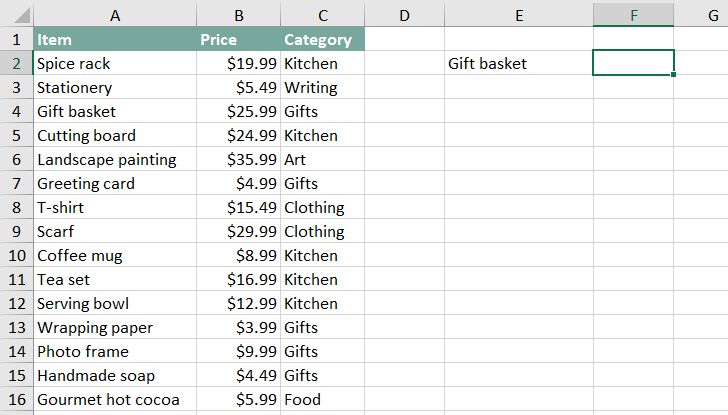
In the previous example, we typed the item name directly into the VLOOKUP formula. But in the real world, you'll usually use a cell reference instead. In this example, we'll type the item name in cell E2, and our VLOOKUP formula can then use a cell reference to find information about that product. Then, we can simply type a new item name into E2 to find any product we want.
We've also added a third column that has the category for each item. This will give us the option of finding the price or category. Here's what the spreadsheet looks like so far:
Our formula will be similar to the previous example, but we'll need to change the first three arguments. Let's start by changing the first argument to a cell reference (make sure to remove the quotation marks):
=VLOOKUP(E2, A2:B16, 2, FALSE)
To find the category, we'll need to change the second and third arguments. First, we'll change the range to A2:C16 so it includes the third column. Next, we'll change the column index number to 3 because our categories are in the third column:
=VLOOKUP(E2, A2:C16, 3, FALSE)
When you press Enter, you'll see that the Gift basket is in the Gifts category.
If we want to find the category of a different item, we can simply change the item name in cell E2:
Try this!
If you'd like more practice, see if you can find the following:
- The price of the coffee mug
- The category of the landscape painting
- The price of the serving bowl
- The category of the scarf
Now that you know the basics of VLOOKUP, you can use it in many different situations. For example, if you have a contact list you could search for someone's name to find his or her phone number. If your contact list has columns for the email address or company name, you could search for those by simply changing the second and third arguments, as we did in our example.
To get even more practice with VLOOKUP, you can check out the Invoice series in our Excel Formulas tutorial. It covers tips for avoiding common problems and using data validation to use VLOOKUP with a drop-down list!