Как посчитать в Excel отклонение в процентах
Привет. Нынешняя статья – не совершенно про Excel, но у меня так нередко требуют совета по данной теме, что я сдался. Потому, рассказываю, как в Экселе посчитать изменение в процентах. Не глядя на видимую простоту темы, тут есть подводные камешки, о которых расскажу.
Обычной расчёт отличия
Основное, что необходимо знать – формула расчета таковая:
Когда вы считаете это в Экселе, программка сама множит число на 100%, когда для ячейки задан процентный формат. Для вас множить не надо. Так, к примеру, в Excel можно вычислить изменение прибыли от реализации продуктов:

Это вправду просто и отлично, пока в расчетах не возникают отрицательные составляющие.
Отклонение в процентах при отрицательных величинах
Что будет с конфигурацией прибыли, если какие-то продукты имеют отрицательное старенькое значение? Пусть в нашем примере в январе мы продавали в убыток и прибыль была негативной. А ведь это не таковой уж и редчайший вариант!

Практически, прибыль выросла, а по расчётам – нет. Исправим формулу, необходимо знаменатель взять по модулю (откинуть символ минус). Это всераспространенный подход, почти все его употребляют. Применим функцию ABS, которая возвращает модуль числа:

Неувязка исправлена, этими плодами можно воспользоваться. Но, желаю вас предостеречь. Результаты могут быть недостаточно корректными. Посмотрите на картину снова. Прибыль от телефонов выросла на 60 тыщ, и это 597%. А прибыль от телевизоров – на 110 тыщ, и это только 183%. Я использую такие результаты только для поверхностной оценки. Либо можно не выводить отклонение для таковых случаев.
Как не считать отклонение в процентах при отрицательных входных параметрах
Вероятное решение описанной чуть повыше трудности – отрешиться от расчёта, когда попадаются нехорошие значения. Создадим это при помощи функции ЕСЛИ:
В этом случае, Эксель будет действовать так:
- При помощи функции МИН, программка отыщет малое число меж старенькым и новеньким значением
- Функция ЕСЛИ проверит, это значение меньше нуля, либо нет? Меньше – выведет на экран надпись «Нет результата». Не меньше – выполнит расчёт по обычной формуле, которую я показал сначала статьи

Вот так обычно считается изменение в процентах. Успешных подсчетов и всего неплохого!
How to calculate the annual growth rate in Excel | Simple formula of percentages

Excel offers us multiple configuration options. As an office automation tool, it allows thousands of calculations to be мейд in just minutes and simplifies day-to-day work tasks. Thanks to Excel, tasks such as calculating the Annual growth rate are very easy to do with percentage formulas .
How do you calculate the annual growth rate in Excel?
Calculating the growth percentages is done automatically and in a very practical way only with the application of formulas. There are many ways to do the calculation, but this is the simplest formula to apply.
- % Growth = ((current value – previous month value) / (previous value)
When applying this formula in Excel in the cell where you want to show the percentage results, the operation will be performed.
- = ((B3-B2) / B2)
B2 represents the value obtained from the previous month, that is, the cell prior to the month being evaluated. Cell B3 represents the current balance, which you want to evaluate the growth percentage.

Note: In order for you to see the percentage value in the cell, you must change the format to percentage. Right click on the cell, select the Cell Format option and finally select the percentage category.
Alternative formula (function TIR.NO.PER or XIRR)
This formula is generally used to evaluate the cash flow value on a regular basis . The meaning of its syntax is TIR.NO.PER and it means “values.dates.estimate”. In case the version of Excel is in English, then the name of the function is XIRR.
- Values: is the range of data used to measure the rate.
- Dates: data evaluation period.
- Estimate : is optional and is used to find an estimated value that is close to the IRR.
All aggregated values must have a minus sign (-) at the end for the calculation to be successful. Applying this formula in Excel would look like this:
- = TIR.NO.PER (B2: B13; C2: C13)
Where column B represents the value and column C represents the date.
Finally, you can calculate the average of the results obtained by comparing the result of a month with other monthly values . It is a default function available and you only access it by writing the average word and placing the values to be calculated.
- = AVERAGE (B2: B13)
Calculation of the average of each month in relation to the total
Once the total sum of all the values to be evaluated has been calculated, the percentage of sales мейд in that period of time in relation to the entire year can be calculated. The formula is just as simple as the one used to calculate the average. The total sum of annual sales is divided by the general total of sales for that month.
- = B2 / $ B $ 14

Note: The sum calculation formula is simple = Sum (B2: B13). What is indicated in this formula is that the sum of all the values between B2 and B3 must be done.
Add graphic icons
To show the results in a more graphic way and that is understandable to the naked eye, you can add colored icons in the shape of an arrow . Each arrow has a meaning, if it is green and up it means that there was a growth in sales, if it is yellow there were no changes with respect to the previous period and if it is red and down it means that there were losses.
To apply this change it is necessary to add one more formula in another cell . The result obtained from the formula is only 1 = there was growth, 0 = remains the same and -1 = there were losses. You must start from the second period, because the first month has no point of comparison.
- = SIGN (B3-B2)
Then select the result obtained in all cells and from the Home tab click on the Conditional Formatting option . Select the icon set you prefer and the changes will be applied immediately.
To remove the numbers next to the icon you must change the formatting rules , from the same Conditional Formatting option you can manage the rules. Select only show symbol, apply the changes and everything will be perfect.