Excel VLOOKUP Function
VLOOKUP is an Excel function to look up data in a table organized vertically. VLOOKUP supports approximate and exact matching, and wildcards (* ?) for partial matches. Lookup values must appear in the first column of the table passed into VLOOKUP.
- value — The value to look for in the first column of a table.
- table — The table from which to retrieve a value.
- col_index — The column in the table from which to retrieve a value.
- range_lookup — [optional] TRUE = approximate match (default). FALSE = exact match.
VLOOKUP is an Excel function to get data from a table organized vertically. Lookup values must appear in the first column of the table passed into VLOOKUP. VLOOKUP supports approximate and exact matching, and wildcards (* ?) for partial matches.
V is for vertical
The purpose of VLOOKUP is to get information from a table organized like this:
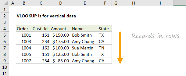
Using the Order number in column B as a lookup value, VLOOKUP can get the Customer ID, Amount, Name, and State for any order. For example, to get the customer name for order 1004, the formula is:
For horizontal data, you can use the HLOOKUP, INDEX and MATCH, or XLOOKUP.
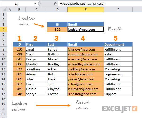
VLOOKUP is based on column numbers
When you use VLOOKUP, imagine that every column in the table is numbered, starting from the left. To get a value from a particular column, provide the appropriate number as the «column index». For example, the column index to retrieve the first name below is 2:
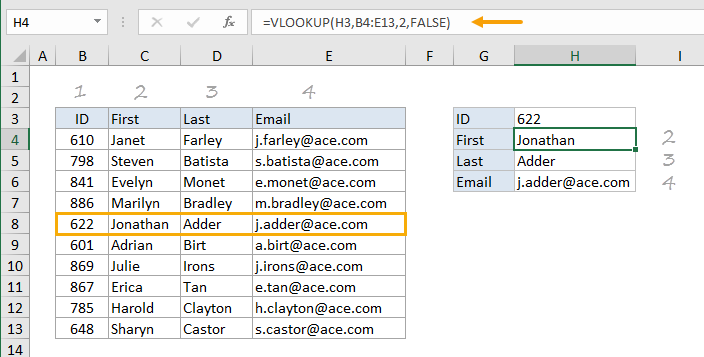
The last name and email can be retrieved with columns 3 and 4:
VLOOKUP only looks right
VLOOKUP can only look to the right. The data you want to retrieve (result values) can appear in any column to the right of the lookup values:
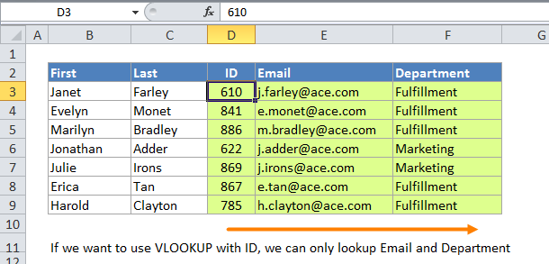
If you need to lookup values to the left, see INDEX and MATCH, or XLOOKUP.
Exact and approximate matching
VLOOKUP has two modes of matching, exact and approximate. The name of the argument that controls matching is «range_lookup«. This is a confusing name, because it seems to have something to do with cell ranges like A1:A10. Actually, the word «range» in this case refers to «range of values» – when range_lookup is TRUE, VLOOKUP will match a range of values rather than an exact value. A good example of this is using VLOOKUP to calculate grades.
It is important to understand that range_lookup defaults to TRUE, which means VLOOKUP will use approximate matching by default, which can be dangerous. Set range_lookup to FALSE to force exact matching:
Note: You can also supply zero (0) instead of FALSE for an exact match.
Exact match
In most cases, you’ll probably want to use VLOOKUP in exact match mode. This makes sense when you have a unique key to use as a lookup value, for example, the movie title in this data:
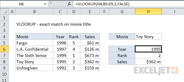
The formula in H6 to find Year, based on an exact match of movie title, is:
Approximate match
In cases when you want the best match, not necessarily an exact match, you’ll want to use approximate mode. For example, below we want to look up a commission rate in the table G5:H10. The lookup values come from column C. In this example, we need to use VLOOKUP in approximate match mode, because in most cases an exact match will never be found. The VLOOKUP formula in D5 is configured to perform an approximate match by setting the last argument to TRUE:
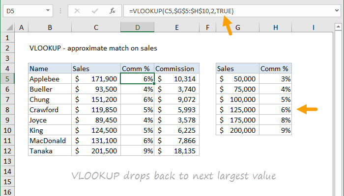
VLOOKUP will scan values in column G for the lookup value. If an exact match is found, VLOOKUP will use it. If not, VLOOKUP will «step back» and match the previous row.
Note: data must be sorted in ascending order by lookup value when you use approximate match mode with VLOOKUP.
First match
In the case of duplicate values, VLOOKUP will find the first match when the match mode is exact. In the screen below, VLOOKUP is configured to find the price for the color «Green». There are three entries with the color Green, and VLOOKUP returns the price for the first entry, $17. The formula in cell F5 is:

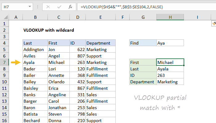
Wildcard match
The VLOOKUP function supports wildcards, which makes it possible to perform a partial match on a lookup value. For instance, you can use VLOOKUP to retrieve values from a table after typing in only part of a lookup value. To use wildcards with VLOOKUP, you must specify the exact match mode by providing FALSE or 0 for the last argument, range_lookup. The formula in H7 retrieves the first name, «Michael», after typing «Aya» into cell H4:
Two-way lookup
Inside the VLOOKUP function, the column index argument is normally hard-coded as a static number. However, you can also create a dynamic column index by using the MATCH function to locate the right column. This technique allows you to create a dynamic two-way lookup, matching on both rows and columns. In the screen below, VLOOKUP is configured to perform a lookup based on Name and Month. The formula in H6 is:

Multiple criteria
The VLOOKUP function does not handle multiple criteria natively. However, you can use a helper column to join multiple fields together, and use these fields like multiple criteria inside VLOOKUP. In the example below, Column B is a helper column that concatenates first and last names together with this formula:
VLOOKUP is configured to do the same thing to create a lookup value. The formula in H6 is:

Note: INDEX and MATCH and XLOOKUP are more robust ways to handle lookups based on multiple criteria.
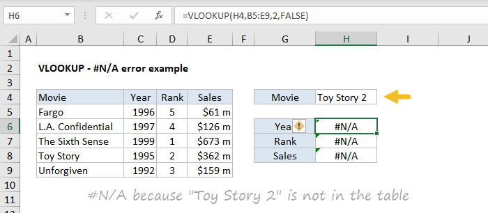
VLOOKUP and #N/A errors
If you use VLOOKUP you will inevitably run into the #N/A error. The #N/A error just means «not found». For example, in the screen below, the lookup value «Toy Story 2» does not exist in the lookup table, and all three VLOOKUP formulas return #N/A:
One way to «trap» the NA error is to use the IFNA function like this:
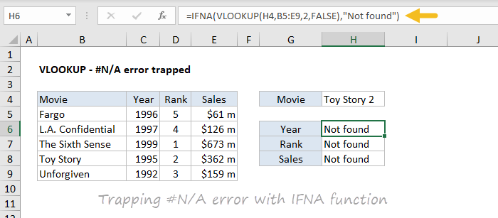
The formula in H6 is:
The message can be customized as desired. To return nothing (i.e. to display a blank result) when VLOOKUP returns #N/A you can use an empty string like this:
The #N/A error is useful because it tells you something is wrong. In practice, there are many reasons why you might see this error, including:
MS Excel: How to use the VLOOKUP Function (WS)
This Excel tutorial explains how to use the VLOOKUP function with syntax and examples.
Description
The VLOOKUP function performs a vertical lookup by searching for a value in the first column of a table and returning the value in the same row in the index_number position.
The VLOOKUP function is a built-in function in Excel that is categorized as a Lookup/Reference Function. It can be used as a worksheet function (WS) in Excel. As a worksheet function, the VLOOKUP function can be entered as part of a formula in a cell of a worksheet.
The VLOOKUP function is actually quite easy to use once you understand how it works! If you want to follow along with this tutorial, download the example spreadsheet.
Syntax
The syntax for the VLOOKUP function in Microsoft Excel is:
Parameters or Arguments
Returns
The VLOOKUP function returns any datatype such as a string, numeric, date, etc.
If you specify FALSE for the approximate_match parameter and no exact match is found, then the VLOOKUP function will return #N/A.
If you specify TRUE for the approximate_match parameter and no exact match is found, then the next smaller value is returned.
If index_number is less than 1, the VLOOKUP function will return #VALUE!.
If index_number is greater than the number of columns in table, the VLOOKUP function will return #REF!.
- See also the HLOOKUP function to perform a horizontal lookup.
Applies To
- Excel for Office 365, Excel 2019, Excel 2016, Excel 2013, Excel 2011 for Mac, Excel 2010, Excel 2007, Excel 2003, Excel XP, Excel 2000
Type of Function
- Worksheet function (WS)
Example (as Worksheet Function)
Let’s explore how to use VLOOKUP as a worksheet function in Microsoft Excel.
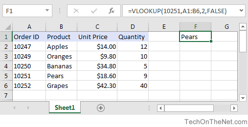
Based on the Excel spreadsheet above, the following VLOOKUP examples would return:
Now, let’s look at the example =VLOOKUP(10251, A1:B6, 2, FALSE) that returns a value of "Pears" and take a closer look why.
First Parameter
The first parameter in the VLOOKUP function is the value to search for in the table of data.
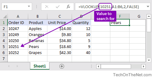
In this example, the first parameter is 10251. This is the value that the VLOOKUP will search for in the first column of the table of data. Because it is a numeric value, you can just enter the number. But if the search value was text, you would need to put it in double quotes, for example:
Second Parameter
The second parameter in the VLOOKUP function is the table or the source of data where the vertical lookup should be performed.
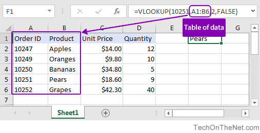
In this example, the second parameter is A1:B6 which gives us two columns to data to use in the vertical lookup — A1:A6 and B1:B6. The first column in the range (A1:A6) is used to search for the Order value of 10251. The second column in the range (B1:B6) contains the value to return which is the Product value.
Third Parameter
The third parameter is the position number in the table where the return data can be found. A value of 1 indicates the first column in the table. The second column is 2, and so on.
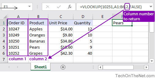
In this example, the third parameter is 2. This means that the second column in the table is where we will find the value to return. Since the table range is set to A1:B6, the return value will be in the second column somewhere in the range B1:B6.
Fourth Parameter
Finally and most importantly is the fourth or last parameter in the VLOOKUP. This parameter determines whether you are looking for an exact match or approximate match.
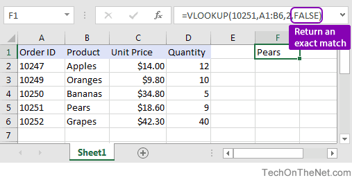
In this example, the fourth parameter is FALSE. A parameter of FALSE means that VLOOKUP is looking for an EXACT match for the value of 10251. A parameter of TRUE means that a "close" match will be returned. Since the VLOOKUP is able to find the value of 10251 in the range A1:A6, it returns the corresponding value from B1:B6 which is Pears.
Exact Match vs. Approximate Match
To find an exact match, use FALSE as the final parameter. To find an approximate match, use TRUE as the final parameter.
Let’s lookup a value that does not exist in our data to demonstrate the importance of this parameter!
Exact Match
Use FALSE to find an exact match:
If no exact match is found, #N/A is returned.
Approximate Match
Use TRUE to find an approximate match:
If no match is found, it returns the next smaller value which in this case is "Apples".
VLOOKUP from Another Sheet
You can use the VLOOKUP to lookup a value when the table is on another sheet. Let’s modify our example above and assume that the table is in a different Sheet called Sheet2 in the range A1:B6.
We could rewrite our original example where we lookup the value 10251 as follows:
By preceding the table range with the sheet name and an exclamation mark, we can update our VLOOKUP to reference a table on another sheet.
VLOOKUP from Another Sheet with Spaces in Sheet Name
Let’s throw in one more complication. What happens if your sheet name contains spaces? If there are spaces in the sheet name, you will need to change the formula further.
Let’s assume that the table is on a Sheet called "Test Sheet" in the range A1:B6, now we need to wrap the Sheet name in single quotes as follows:
By placing the sheet name within single quotes, we can handle a sheet name with spaces in the VLOOKUP function.
VLOOKUP from Another Workbook
You can use the VLOOKUP to lookup a value in another workbook. For example, if you wanted to have the table portion of the VLOOKUP formula be from an external workbook, we could try the following formula:
This would look for the value 10251 in the file C:data.xlxs in Sheet 1 where the table data is found in the range $A$1:$B$6.
Why use Absolute Referencing?
Now it is important for us to cover one more mistake that is commonly мейд. When people use the VLOOKUP function, they commonly use relative referencing for the table range like we did in some of our examples above. This will return the right answer, but what happens when you copy the formula to another cell? The table range will be adjusted by Excel and change relative to where you paste the new formula. Let’s explain further.
So if you had the following formula in cell G1:
And then you copied this formula from cell G1 to cell H2, it would modify the VLOOKUP formula to this:
Since your table is found in the range A1:B6 and not B2:C7, your formula would return erroneous results in cell H2. To ensure that your range is not changed, try referencing your table range using absolute referencing as follows:
Now if you copy this formula to another cell, your table range will remain $A$1:$B$6.
How to Handle #N/A Errors
Next, let’s look at how to handle instances where the VLOOKUP function does not find a match and returns the #N/A error. In most cases, you don’t want to see #N/A but would rather display a more user-friendly result.
For example, if you had the following formula:
Instead of displaying #N/A error if you do not find a match, you could return the value "Not Found". To do this, you could modify your VLOOKUP formula as follows:
These formulas use the ISNA, IFERROR and IFNA functions to return "Not Found" if a match is not found by the VLOOKUP function.
This is a great way to spruce up your spreadsheet so that you don’t see traditional Excel errors.
Frequently Asked Questions
If you want to find out what others have asked about the VLOOKUP function, go to our Frequently Asked Questions.