КАК: Учебник по Excel CHOOSE — 2021
Отыскать посреди чисел лишь те, которые составляют обозначенную сумму (Октябрь 2021).
Table of Contents:
Функция CHOOSE Excel употребляет номер индекса для поиска и возврата определенного значения из соответственного перечня данных. Номер индекса показывает позицию значения в перечне.
Заметка: Информация в данной для нас статье относится к Excel 2019, Excel 2016, Excel 2013, Excel 2010, Excel 2019 для Mac, Excel 2016 для Mac, Excel для Mac 2011 и Excel Online.
ВЫБРАТЬ Обзор функций

Как и почти все функции Excel, CHOOSE более эффективен, когда он смешивается с иными формулами либо функциями, чтоб возвращать различные результаты.
Примером быть может внедрение CHOOSE для выполнения вычислений с внедрением функций SUM, AVERAGE либо MAX из Excel по этим же данным в зависимости от избранного номера индекса.
Синтаксис и аргументы CHOOSE
Синтаксис функции относится к компоновке функции и включает имя функции, скобки и аргументы.
Синтаксис функции CHOOSE:
= ВЫБРАТЬ (номер_индекса,Значение1,Value2,…Value254)
номер_индекса (непременно): Описывает, какое значение обязано быть возвращено функцией. Index_num быть может числом от 1 до 254, формулой либо ссылкой на ячейку, содержащую число от 1 до 254.
Значение (Требуется значение 1. Доп значения, максимум 254, являются необязательными): Перечень значений, возвращаемых функцией в зависимости от аргумента Index_num. Значения могут быть числами, ссылками на ячейки, именованными спектрами, формулами, функциями либо текстом.
Пример использования функции CHOOSE в Excel для поиска данных

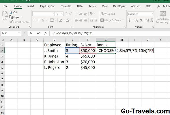
Чтоб проиллюстрировать, как употреблять функцию CHOOSE, следуйте вкупе с примером, применяемым в этом руководстве. В нашем примере мы используем функцию CHOOSE для расчета годичного приза для служащих.
Приз — это процентная ставка от годичного оклада, а процентная ставка зависит от рейтинга производительности от 1 до 4.
Функция CHOOSE конвертирует рейтинг производительности в верный процент:
Рейтинг 1: 3% Рейтинг 2: 5% Рейтинг 3: 7% Рейтинг 4: 10%
Потом это процентное значение множится на годичный оклад, чтоб отыскать годичный приз сотрудника.
В этом примере показано, как ввести функцию CHOOSE в ячейку G2, а потом употреблять дескриптор наполнения для копирования функции в ячейки G2-G5.
Введите данные учебника
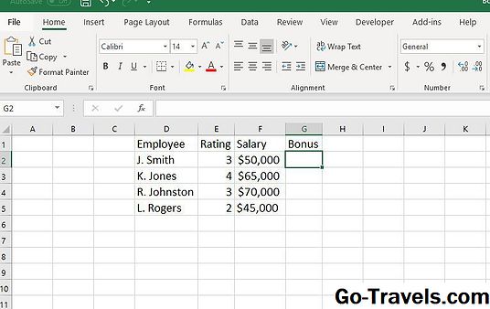
Введите последующие данные в ячейки D1-G1:
- Cell D1: Сотрудник
- Cell D2: J. Smith
- Ячейка D3: К. Джонс
- Ячейка D4: Р. Джонстон
- Ячейка D5: Л. Роджерс
- Ячейка E1: Рейтинг
- Ячейка E2: 3
- Ячейка E3: 4
- Ячейка E4: 3
- Ячейка E5: 2
- Ячейка F1: Заработная плата
- Cell F2: 50 000 баксов США (Соединённые Штаты Америки — государство в Северной Америке)
- Cell F3: 65 000 баксов США (Соединённые Штаты Америки — государство в Северной Америке)
- Cell F4: 70 000 баксов США (Соединённые Штаты Америки — государство в Северной Америке)
- Cell F5: 45 000 $
- Ячейка G1: Приз
Введите функцию ВЫБОР

Этот раздел управления вводит функцию CHOOSE в ячейку G2 и вычисляет процент приза в зависимости от рейтинга производительности для первого сотрудника. Эти шаги используются к Excel 2019, Excel 2016, Excel 2013, Excel 2010 и Excel для Mac.
- Избрать ячейку G2, Тут будут отображаться результаты функции.
- Изберите Формулы Вкладка.
- изберите Поиск и ссылки чтоб открыть раскрывающийся перечень функций.
- Избрать ВЫБИРАТЬ в перечне, чтоб вызвать диалоговое окно «Аргументы функций».
- Расположите курсор в номер_индекса в диалоговом окне.
- Избрать ячейку E2 на листе, чтоб ввести ссылку на ячейку в диалоговом окне.
- Расположите курсор в Значение1 в диалоговом окне.
- Войти 3% на данной для нас полосы.
- Расположите курсор в Value2 в диалоговом окне.
- Войти 5% на данной для нас полосы.
- Расположите курсор в Value3 в диалоговом окне.
- Войти 7% на данной для нас полосы.
- Расположите курсор в Value4 в диалоговом окне.
- Войти 10% на данной для нас полосы.
- Избрать Отлично для окончания функции и закрытия диалогового окна
Значение 0.07 возникает в ячейке G2, которая является десятичной формой для 7%.
В Excel Online нет вкладки «Формула». Заместо этого используйте клавишу «Вставить функцию», чтоб ввести функцию CHOOSE в Excel Online либо всякую другую версию Excel.
- Избрать ячейку G2, Тут будут отображаться результаты функции.
- Избрать Вставить функцию рядом с панелью формул.
- изберите Поиск и ссылки из перечня категорий.
- Избрать ВЫБИРАТЬ в перечне и изберите Отлично.
- Тип (E2,3%, 5%, 7%, 10%) опосля = ВЫБРАТЬ в строке формул. Непременно укажите круглые скобки.
- Нажмите Войти.
Значение 0.07 возникает в ячейке G2, которая является десятичной формой для 7%.
Вычислить приз сотрудника
Сейчас вы сможете поменять функцию CHOOSE в ячейке G2, умножив результаты функции на годичный оклад сотрудника, чтоб высчитать собственный годичный приз.
Эта модификация производится при помощи клавиши F2 для редактирования формулы.
- Избрать ячейку G2 создать его активной ячейкой
- Нажмите F2 для размещения Excel в режиме редактирования. Полная функция,= CHOOSE (E2,3%, 5%, 7%, 10%), возникает в ячейке с точкой вставки, расположенной опосля закрывающей скобки функции.
- Введите звездочку ( * ), знак умножения в Excel, опосля закрывающей скобки.
- Избрать ячейку F2 на листе, чтоб ввести ссылку ячейки на годичный оклад работника в формулу.
- Нажмите Войти для окончания формулы и выхода из режима редактирования.
- Значение в размере 3 500 баксов США (Соединённые Штаты Америки — государство в Северной Америке) возникает в ячейке G2, что составляет 7% от годичного оклада сотрудника в размере 50 000,00 баксов США (Соединённые Штаты Америки — государство в Северной Америке).
- Избрать ячейку G2. Полная формула = CHOOSE (E2,3%, 5%, 7%, 10%) * F2 возникает в строке формул, расположенной над листом.
Скопируйте Формулу Приза Сотрудника при помощи Заливной Ручки

Крайний шаг — скопировать формулу в ячейку G2 в ячейки G3-G5 при помощи дескриптора наполнения.
- Избрать ячейку G2 чтоб создать его активной ячейкой.
- Расположите указатель мыши на темный квадрат в нижнем правом углу ячейки G2. Указатель изменяется на символ плюса (+).
- Перетащите дескриптор наполнения в ячейку G5.
- Ячейки G3-G5 содержат бонусные характеристики для других служащих.
Учебник Excel — преобразование таблицы для доступа к базе данных 2010
Учебник Excel — преобразование таблицы для доступа к базе данных 2010
Excel 2003 Линейный графический иллюстрированный учебник
В этом руководстве описывается создание линейного графика в версиях Microsoft Excel прямо до Excel 2003. Учебное пособие включает пошаговый пример.
Учебник по форме ввода данных Excel

В этом учебном пособии описывается внедрение формы ввода данных для прибавления данных в базу данных в Excel. Включен пошаговый пример того, как сделать форму.
Excel CHOOSE function with formula examples
CHOOSE is one of those Excel functions that may not look useful on their own, but combined with other functions give a number of awesome benefits. At the most basic level, you use the CHOOSE function to get a value from a list by specifying the position of that value. Further on in this tutorial, you will find several advanced uses that are certainly worth exploring.
Excel CHOOSE function — syntax and basic uses
The CHOOSE function in Excel is designed to return a value from the list based on a specified position.
The function is available in Excel 365, Excel 2019, Excel 2016, Excel 2013, Excel 2010, and Excel 2007.
The syntax of the CHOOSE function is as follows:
Index_num (required) — the position of the value to return. It can be any number between 1 and 254, a cell reference, or another formula.
Value1, value2, … — a list of up to 254 values from which to choose. Value1 is required, other values are optional. These can be numbers, text values, cell references, formulas, or defined names.
Here’s an example of a CHOOSE formula in the simplest form:
=CHOOSE(3, «Mike», «Sally», «Amy», «Neal»)
The formula returns «Amy» because index_num is 3 and «Amy» is the 3 rd value in the list:
Excel CHOOSE function — 3 things to remember!
CHOOSE is a very plain function and you will hardly run into any difficulties implementing it in your worksheets. If the result returned by your CHOOSE formula is unexpected or not the result you were looking for, it may be because of the following reasons:
- The number of values to choose from is limited to 254.
- If index_num is less than 1 or greater than the number of values in the list, the #VALUE! error is returned.
- If the index_num argument is a fraction, it is truncated to the lowest integer.
How to use CHOOSE function in Excel — formula examples
The following examples show how CHOOSE can extend the capabilities of other Excel functions and provide alternative solutions to some common tasks, even to those that are considered unfeasible by many.
Excel CHOOSE instead of nested IFs
One of the most frequent tasks in Excel is to return different values based on a specified condition. In most cases, this can be done by using a classic nested IF statement. But the CHOOSE function can be a quick and easy-to-understand alternative.
Example 1. Return different values based on condition
Supposing you have a column of student scores and you want to label the scores based on the following conditions:
| Result | Score |
| Poor | 0 — 50 |
| Satisfactory | 51 — 100 |
| Good | 101 — 150 |
| Excellent | over 151 |
One way to do this is to nest a few IF formulas inside each other:
=IF(B2>=151, «Excellent», IF(B2>=101, «Good», IF(B2>=51, «Satisfactory», «Poor»)))
Another way is to choose a label corresponding to the condition:
=CHOOSE((B2>0) + (B2>=51) + (B2>=101) + (B2>=151), «Poor», «Satisfactory», «Good», «Excellent»)
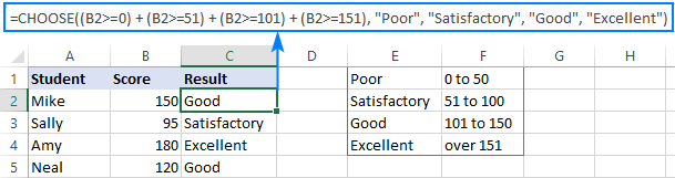
How this formula works:
In the index_num argument, you evaluate each condition and return TRUE if the condition is met, FALSE otherwise. For example, the value in cell B2 meets the first three conditions, so we get this intermediate result:
=CHOOSE(TRUE + TRUE + TRUE + FALSE, «Poor», «Satisfactory», «Good», «Excellent»)
Given that in most Excel formulas TRUE equates to 1 and FALSE to 0, our formula undergoes this transformation:
=CHOOSE(1 + 1 + 1 + 0, «Poor», «Satisfactory», «Good», «Excellent»)
After the addition operation is performed, we have:
=CHOOSE(3, «Poor», «Satisfactory», «Good», «Excellent»)
As the result, the 3 rd value in the list is returned, which is «Good».
-
To make the formula more flexible, you can use cell references instead of hardcoded labels, for example:
Example 2. Perform different calculations based on condition
In a similar fashion, you can use the Excel CHOOSE function to perform one calculation in a series of possible calculations/formulas without nesting multiple IF statements inside each other.
As an example, let’s calculate the commission of each seller depending on their sales:
| Commission | Sales |
| 5% | $0 to $50 |
| 7% | $51 to $100 |
| 10% | over $101 |
With the sales amount in B2, the formula takes the following shape:
=CHOOSE((B2>0) + (B2>=51) + (B2>=101), B2*5%, B2*7%, B2*10%)
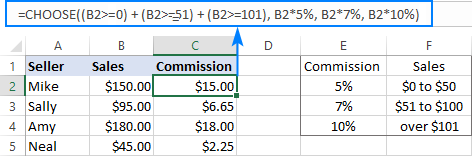
Instead of hardcoding the percentages in the formula, you can refer to the corresponding cell in your reference table, if there is any. Just remember to fix the references using the $ sign.
=CHOOSE((B2>0) + (B2>=51) + (B2>=101), B2*$E$2, B2*$E$3, B2*$E$4)
Excel CHOOSE formula to generate random data
As you probably know, Microsoft Excel has a special function to generate random integers between the bottom and top numbers that you specify — RANDBETWEEN function. Nest it in the index_num argument of CHOOSE, and your formula will generate almost any random data you want.
For example, this formula can produce a list of random exam results:
=CHOOSE(RANDBETWEEN(1,4), «Poor», «Satisfactory», «Good», «Excellent»)
The formula’s logic is obvious: RANDBETWEEN generates random numbers from 1 to 4 and CHOOSE returns a corresponding value from the predefined list of four values.
CHOOSE formula to do a left Vlookup
If you have ever performed a vertical lookup in Excel, you know that the VLOOKUP function can only search in the left-most column. In situations when you need to return a value to the left of the lookup column, you can either use the INDEX / MATCH combination or trick VLOOKUP by nesting the CHOOSE function into it. Here’s how:
Supposing you have a list of scores in column A, student names in column B, and you want to retrieve a score of a particular student. Since the return column is to the left of the lookup column, a regular Vlookup formula returns the #N/A error:
To fix this, get the CHOOSE function to swap the positions of columns, telling Excel that column 1 is B and column 2 is A:
Because we supply an array of <1,2>in the index_num argument, the CHOOSE function accepts ranges in the value arguments (normally, it doesn’t).
Now, embed the above formula into the table_array argument of VLOOKUP:
=VLOOKUP(E1,CHOOSE(<1,2>, B2:B5, A2:A5),2,FALSE)
And voilà — a lookup to the left is performed without a hitch!
CHOOSE formula to return next working day
If you are not sure whether you should go to work tomorrow or can stay at home and enjoy your well-deserved weekend, the Excel CHOOSE function can find out when the next work day is.
Assuming your working days are Monday to Friday, the formula goes as follows:
Tricky at first sight, upon a closer look the formula’s logic is easy to follow:
WEEKDAY(TODAY()) returns a serial number corresponding to today’s date, ranging from 1 (Sunday) to 7 (Saturday). This number goes to the index_num argument of our CHOOSE formula.
Value1 — value7 (1,1,1,1,1,3,2) determine how many days to add to the current date. If today is Sunday — Thursday (index_num 1 — 5), you add 1 to return the next day. If today is Friday (index_num 6), you add 3 to return next Monday. If today is Saturday (index_num 7), you add 2 to return next Monday again. Yep, it’s that simple 🙂
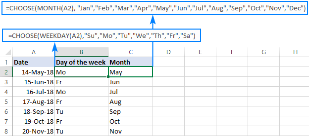
CHOOSE formula to return a custom day/month name from date
In situations when you want to get a day name in the standard format such as full name (Monday, Tuesday, etc.) or short name (Mon, Tue, etc.), you can use the TEXT function as explained in this example: Get day of week from date in Excel.
If you wish to return a day of the week or a month name in a custom format, use the CHOOSE function in the following way.
To get a day of the week:
Where A2 is the cell containing the original date.
I hope this tutorial has given you some ideas of how you can use the CHOOSE function in Excel to enhance your data models. I thank you for reading and hope to see you on our blog next week!
Download practice workbook
You may also be interested in
26 comments to «Excel CHOOSE function with formula examples»
How to write 24% in another line with text & column picked.
24% Increase in Past dues by 0.241101852425452
Create an efficient formula in range G2:G21 that gives a decision for each customer with either the text “Extend Credit” or “No Credit.” Copy this formula down for each customer.
What formula would I use? How to enter in cell «Extend Credit» or «No credit»?
Kindly help to use choose in vlookup function
i have two cells in my excel that is prepared for one particular location to the other e.g france to italy. how can i make the next cell pick the distance between the two location.
1 Count
2 Average
3 Sum
4 Max
5 Min
Based on the selection in the cell below, that function should be applied to output for Qty & Sales column
Function Qty Sales
2
Order ID Order Date Customer Name Region Customer Segment Product Category Product Sub-Category Product Name Order Quanqtity Unit Price Sales Order Priority Product Container
1001 1-Mar-17 Roy Skaria West Corporate Technology Computer Peripherals Zoom V.92 USB External Faxmodem 45 3000 135000 Low Large Box
1002 1-Mar-17 Roy Skaria West Corporate Office Supplies Paper Unpadded Memo Slips 50 240 12000 Low Jumbo Drum
1003 2-Mar-17 Roy Skaria North Corporate Office Supplies Pens & Art Supplies Prismacolor Color Pencil Set 10 1200 12000 Medium Small Box
1004 2-Mar-17 Dario Medina East Small Business Office Supplies Storage & Organization Sterilite Officeware Hinged File Box 27 660 17820 Critical Small Box
1005 2-Mar-17 Resi Polking West Small Business Technology Copiers and Fax Canon PC-428 Personal Copier 38 12000 456000 Medium Medium Box
1006 3-Mar-17 Ralph Knight North Consumer Technology Telephones and Communication 600 Series Flip 14 5760 80640 Medium Small Pack
1007 3-Mar-17 Deborah Brumfield North Corporate Furniture Chairs & Chairmats Hon GuestStacker Chair 25 13620 340500 Low Small Box
1008 3-Mar-17 Eva Jacobs East Home Office Technology Office Machines Lexmark Z54se Color Inkjet Printer 26 5460 141960 Low Small Box
1009 3-Mar-17 Jill Matthias West Consumer Technology Office Machines Polycom ViewStation™ Adapter H323 Videoconferencing Unit 2 116341 232682 Medium Large Box
calculate
Count
Average
Sum
Max
Min
funtion is a scrolling bar.
Greeting Sir,
it giving me error
Hello!
I’m sorry but your task is not entirely clear to me. For me to be able to help you better, please describe your task in more detail. Please specify what you were trying to find, what formula you used and what problem or error occurred. Give an example of the source data and the expected result.
It’ll help me understand it better and find a solution for you. Thank you.
Incentive Calls Target
Not Applicable >50
5₹ 50 to 100
7₹ 101 to 201
10₹ over 202
A agent is taking 300 call in a month.How much will be total money?
How to calculate incentive by formula in Excel.
I JUST LOVED THE WAY YOU EXPLAIN & SIMPLIFY THE EXCEL TO THE LEARNERS
THANKS A LOTT FOR YOUR PRECIOUS HELP.