How to Use Excel MOD Function (Examples Video)
How to Use Excel MOD Function (Examples + Video)

MOD function can be used when you want to get the remainder when one number is divided by another number.
What it Returns
It returns a numerical value that represents the remainder when one number is divided by another.
Syntax
Input Arguments
- number – A numeric value for which you want to find the remainder.
- divisor – A number with which you want to divide the number argument. If the divisor is 0, then it will return the #DIV/0! error.
Additional Notes
- If the divisor is 0, then it will return the #DIV/0! error.
- The result always has the same sign as that of the divisor.
- You can use decimal numbers in the MOD function. For example, if you use the function =MOD(10.5,2.5), it will return 0.5.
Examples of Using MOD Function in Excel
Here are useful examples of how you can use the MOD function in Excel.
Example 1 – Add Only the Odd or the Even Numbers
Suppose you have a dataset as shown below:
Here is the formula you can use to add only the even numbers:
Note that here I have hard coded the range ($A$2:$A$11). If your data is likely to change, you can use an Excel Table or created a dynamic named range.
Similarly, if you want to add only the odd numbers, use the below formula:

This formula works by calculating the remainder using the MOD function.
For example, when calculating the sum of odd numbers, (MOD($A$2:$A$11,2)=1) would return an array of TRUEs and FALSEs. If the number is odd, it would return a TRUE, else a FALSE.
SUMPRODUCT function then only adds those numbers that are returning a TRUE (i.e., odd numbers).
The same concept works when calculating the sum of even numbers.
Example 2 – Specify a Number in Every Nth Cell
Suppose you are making a list of fix expenses every month as shown below:
While the house and car EMIs are monthly, the insurance premium is paid every three months.
You can use the MOD function to quickly fill the cell in every third row with the EMI value.
Here is the formula that will do this:

This formula simply analyzes the number given by ROW()-1.
ROW function gives us the row number and we have subtracted 1 as our data starts from second row onwards. Now the MOD function checks the remainder when this value is divided by 3.
It will be 0 for every third row. Whenever this is the case, IF function would return 457, else it will return a blank.
Example 3 – Highlight Alternate Rows in Excel
Highlighting alternate rows can increase the readability of your data set (especially when it’s printed).
Something as shown below:
Note that every second row of the dataset is highlighted.
While you can do this manually for a small dataset, if you have a huge one, you can leverage the power of conditional formatting with the MOD function.
Here are the steps that will highlight every second row in the dataset:
- Select the entire data set.
- Go to the Home tab.
- Click on Conditional Formatting and select New Rule.
- In the ‘New Formatting Rule’ dialog box, select ‘Use a formula to determine which cells to format’.
- In the formula field, enter the following formula: =MOD(ROW()-1,2)=0

- Click on the Format button and specify the color in which you want the rows highlighted.
- Click OK.

This will instantly highlight alternate rows in the dataset.
You can read more about this technique and variations of it in this tutorial.
Example 4 – Highlight All the Integer /Decimal Values
You can use the same conditional formatting concept shown above to highlight integer values or decimal values in a data set.
For example, suppose you have a dataset as shown below:

There are numbers that are integers and some of these have decimal values as well.
Here are the steps to highlight all the numbers that have decimal value in it:
- Select the entire data set.
- Go to the Home tab.
- Click on Conditional Formatting and select New Rule.
- In the ‘New Formatting Rule’ dialog box, select ‘Use a formula to determine which cells to format’.
- In the formula field, enter the following formula: =MOD(A1,1)<>0
- Click on the Format button and specify the color in which you want the rows highlighted.
- Click OK.
This will highlight all the numbers that have a decimal part to it.

Note that we in this example, we have used the formula =MOD(A1,1)<>0. In this formula, make sure the cell reference is absolute (i.e., A1) and not relative (i.e., it shouldn’t be $A$1, $A1 or A$1).
Excel MOD Function – Video Tutorial
Excel MOD Function

The Excel MOD function returns the remainder of two numbers after division. For example, MOD(10,3) = 1. The result of MOD carries the same sign as the divisor.
- number — The number to be divided.
- divisor — The number to divide with.
The MOD function returns the remainder after division. For example, MOD(3,2) returns 1, because 2 goes into 3 once, with a remainder of 1.
The MOD function takes two arguments: number and divisor. Number is the number to be divided, and divisor is the number used to divide. Both arguments are required. If either argument is not numeric, the MOD function returns #VALUE!.
Equation
The result from the MOD function is calculated with an equation like this:
where n is number, d is divisor, and INT is the INT function. This can create some unexpected results because of the way that the INT function rounds negative numbers down, way from zero:
MOD with negative numbers is implemented differently in different languages.
Examples
Below are some examples of the MOD function with hardcoded values:
Negative numbers
The result from MOD carries the same sign as divisor. If divisor is positive, the result from MOD is positive, if divisor is negative, the result from MOD is negative:
Time from datetime
The MOD function can be used to extract the time value from an Excel date that includes time (sometimes called a datetime). With a datetime in A1, the formula below returns the time only:
Large numbers
With very large numbers, you may see the MOD function return a #NUM error. In that case, you can try an alternative version based on the INT function:
Функция ОСТАТ в Excel
(получение остатка от деления)
Функция ОСТАТ в Excel создана для получения остатка от деления 1-го числа на другое. Относится к группе математических формул программки, применять которую весьма просто (смотрите описание функции ОСТАТ, также примеры и видео-урок).
Получение остатка от деления мы все помним ещё со школы. Ну хорошо, по правде сказать почти все это уже запамятовали. В любом случае на данный момент придётся это вспомянуть, если Вы желаете осознавать, как работает функция ОСТАТ в Excel.
Заглавие функции ОСТАТ происходит в Excel от «остаток», так что уяснить просто.
В принципе, сложного ничего нет, но всё же поначалу разглядим синтаксис функции и индивидуальности её работы, если таковые найдутся.
Синтаксис функции ОСТАТ в Excel
Чтоб получить остаток от деления, до этого всего необходимо выполнить саму операцию деления. И хотя на данный момент нам нужен лишь остаток, для его получения необходимо передать в формулу два аргумента, причём оба будут неотклонимыми.
В обобщённом виде синтаксис смотрится так:
ОСТАТ(число; делитель)
Аргументы имеют последующее значение:
- число — Число, остаток от деления которого требуется найти.
- делитель — Число, на которое необходимо поделить (делитель).
Так как тут имеет пространство операция деления, то 2-ой аргумент не быть может равным нулю, по другому мы получим ошибку «#ДЕЛ/0!». Обработать эту и остальные ошибки Для вас поможет формула ЕСЛИОШИБКА. Также в функцию недозволено передавать значения, не являющиеся числами.
Остальных особенностей получение остатка от деления в Excel нет.
Примеры получения остатка от деления
Для примера скопируйте выражение «=ОСТАТ(10; 2)» в пустую ячейку таблицы. В итоге вычисления получим ноль, поэтому что 10 делится на 2 без остатка. Если 1-ый аргумент поменять на 11, то мы получим уже единицу в качестве остатка, потому что 10 делится на 2, а остаётся ещё единица до 11-ти.
Другие примеры можно поглядеть в прикреплённом файле Excel опосля статьи, также на видео.
Если способны к самообучению и желаете научиться работать в Excel, то советуем направить внимание на наш спецкурс по данной программке. Примеры уроков и описание видеокурса есть тут.
Глядеть видео
Функция ОСТАТ в Excel
(получение остатка от деления)

Прикреплённые документы
Вы сможете просмотреть хоть какой прикреплённый документ в виде PDF файла. Все документы открываются во всплывающем окне, потому для закрытия документа пожалуйста не используйте клавишу «Вспять» браузера.
- Справка по функции ОСТАТ в Excel.pdf
Файлы для загрузки
Вы сможете скачать прикреплённые ниже файлы для ознакомления. Обычно тут располагаются разные документы, также остальные файлы, имеющие конкретное отношение к данной публикации.