КАК: Функция Excel SUMIF добавляет значения, надлежащие аспектам — 2021

Learn Python — Full Course for Beginners [Tutorial] (Октябрь 2021).

SUMIF функция соединяет воединыждыЕСЛИ такжеSUM функции в Excel; эта композиция дозволяет добавлять значения в избранный спектр данных, соответственных определенным аспектам. ЕСЛИ часть функции описывает, какие данные соответствуют обозначенным аспектам, и SUM часть делает дополнение.

Обычно, SUMIF употребляется с строчками данных, именуемыми учет, В записи все данные в каждой ячейке в строке соединены — к примеру, имя компании, адресок и номер телефона. SUMIF отыскивает определенные аспекты в одной ячейке либо поле в записи, и, если он находит совпадение, он добавляет данные либо данные в другое данное поле в одной записи.

Синтаксис функции SUMIF

В Excel синтаксис функции относится к компоновке функции и включает имя, скобки и аргументы функции. Синтаксис для SUMIF функция:

= SUMIF (Спектр, Аспекты, Sum_range)

Аргументы функции указывают функции, для какого условия мы тестируем и какой спектр данных суммируем при выполнении условия.

Диапазон: Группу ячеек делает функция поиска.

Аспекты:Значение, которое необходимо сопоставить с данными в Диапазон клеточки. Если совпадение найдено, то надлежащие данные в суммарный_диапазон добавляется. Для этого аргумента можно ввести фактические данные либо ссылку на ячейки для данных.

Диапазон_суммирования (необязательно): данные в этом спектре ячеек складываются, когда совпадения найдены меж диапазон аргумента и аспекты, Если этот спектр опущен, 1-ый спектр суммируется.

Продолжить чтение ниже

Ввод данных учебника

В этом руководстве употребляется набор записей данных и SUMIF чтоб отыскать общие годичные реализации для торговых представителей, которые продали наиболее 250 заказов. Следуя инструкциям, приведенным ниже, вы сможете сделать и применять SUMIF функцию, показанную на изображении выше, для расчета общего годичного размера продаж.

1-ый шаг к использованию SUMIF функция в Excel — это ввести данные. Введите данные в ячейки B1 в E11 листа Excel, как показано на изображении выше. SUMIF функция и аспекты поиска (наиболее 250 заказов) будут добавлены к строке 12 ниже данных.

В инструкциях по обучению не указаны шаги форматирования для рабочего листа. Это не помешает окончить учебное пособие. Ваш рабочий лист будет смотреться по другому, чем показано на примере. SUMIF функция даст для вас те же результаты.

Продолжить чтение ниже

Пуск функции SUMIF

Хотя можно просто набрать SUMIF функции в ячейку на листе, почти всем людям проще применять Formula Builder для входа в функцию.

Нажмите на клеточка E12 создать его активной ячейкой — вот где мы войдем в SUMIF функция.
Нажми на Вкладка «Формулы».
Нажми на Math & Trig на ленте, чтоб открыть Formula Builder.
Нажмите на SUMIF в перечне, чтоб начать создание функции.

Данные, которые мы вводим в три пустые строчки в диалоговом окне, образуют аргументы SUMIF функция; эти аргументы молвят функции, какое условие мы тестируем и какой спектр данных суммируем при выполнении условия.

Ввод спектра и критериев

В этом уроке мы желаем отыскать общий размер продаж для тех торговых представителей, у каких было наиболее 250 заказов в год. Аргумент Range показывает SUMIF функцию, которую группа ячеек обязана находить, пытаясь отыскать обозначенные аспекты > 250.

в Formula Builder, нажми на Диапазон линия.
главный момент ячейки D3 в D9 на листе для ввода этих ссылок на ячейки в качестве спектра для поиска функцией.
Нажми на аспекты линия.
Нажмите на клеточка E13 для ввода данной нам ссылки на ячейку. Функция будет находить спектр, избранный на прошлом шаге, для данных, соответственных этому аспекту (север).

В этом примере, если данные в спектре D3: D12 превосходит 250, тогда общие реализации для данной нам записи будут добавлены SUMIF функция.

Хотя фактические данные — к примеру, текст либо числа, такие как > 250 можно ввести в диалоговое окно для этого аргумента, обычно идеальнее всего добавить данные в ячейку на листе и потом ввести эту ссылку на ячейку в диалоговом окне.

Ссылки на ячейки Прирастить функциональность

Если ссылка на ячейку, к примеру E12, вводится как Аргумент Аспект, SUMIF функция будет находить совпадения с тем, какие данные были введены в эту ячейку на листе.

Таковым образом, опосля нахождения общих продаж для Sales Reps с наиболее чем 250 заказами, будет просто отыскать общий размер продаж для остальных номеров заказов, таковых как наименее 100, просто методом конфигурации > 250 в 250 в D12 — ячейка, идентифицированная в функции, содержащая аргумент критериев.

В ячейка D12 тип > 250 и нажмите Войти на клавиатуре.
Ответ $290,643.00 должен показаться в ячейка E12.
Когда вы нажимаете ячейка E12, полная функция, как показано выше, возникает в строке формул над листом.

Интересно почитать: Функция сегодня в excel примеры

Аспект > 250 производится в 4 ячейках в столбец D: D4, D5, D8, D9, В итоге числа в соответственных ячейках в столбце E: E4, E5, E8, E9 суммируются.

Чтоб отыскать общую сумму продаж для различных порядков, введите сумму в ячейка E12 и нажмите Войти на клавиатуре. Потом общий размер продаж соответственного количества ячеек должен показаться в ячейка E12.

Ячейки сумм, которые удовлетворяют нескольким аспектам при помощи Excel SUMPRODUCT

Используйте функцию SUMPRODUCT в Excel для суммирования значений ячеек, соответственных нескольким аспектам. Врубается шаг за шагом.

Yamaha добавляет цифровой звуковой проектор YSP-5600 с поддержкой Dolby Atmos

Нереально решить меж ресивером / динамиком домашнего кинозала и звуковой панелью? Ознакомьтесь с цифровым звуковым проектором YSP-5600 с поддержкой Dolby Atmos от Yamaha.

Amazon добавляет сенсорный экран в считыватель Kindle Reader

Amazon модернизирует собственный Kindle с исходным уровнем с сенсорным интерфейсом, сохраняя при всем этом стоимость ниже 100 баксов.

SUMIF Function

The SUMIF function is categorized under Excel Math and Trigonometry functions Functions List of the most important Excel functions for financial analysts. This cheat sheet covers 100s of functions that are critical to know as an Excel analyst . It will sum up cells that meet the given criteria. The criteria are based on dates, numbers, and text. It supports logical operators such as (>, <, <>, =) and also wildcards (*, ?). This guide to the SUMIF Excel function will show you how to use it, step-by-step.

As a financial analyst Financial Analyst Job Description The financial analyst job description below gives a typical example of all the skills, education, and experience required to be hired for an analyst job at a bank, institution, or corporation. Perform financial forecasting, reporting, and operational metrics tracking, analyze financial data, create financial models , SUMIF is a frequently used function. Suppose we are given a table listing the consignments of vegetables from different suppliers. The names of the vegetable, names of suppliers, and quantity are in column A, column B, and column C, respectively. In such a scenario, we can use the SUMIF function to find out the sum of the amount related to a particular vegetable from a specific supplier.

Formula

=SUMIF(range, criteria, [sum_range])

The formula uses the following arguments:

Range (required argument) – This is the range of cells that we want to apply the criteria against.
Criteria (required argument) – This is the criteria which are used to determine which cells need to be added.

When we provide the criteria argument, it can either be:

A numeric value (which may be an integer, decimal, date, time, or logical value) (e.g. 10, 01/01/2018, TRUE) or
A text string (e.g. “Text”, “Thursday”) or
An expression (e.g. “>12”, “<>0”).

Sum_range (optional argument) – This is an array of numeric values (or cells containing numeric values) that are to be added together if the corresponding range entry satisfies the supplied criteria. If the [sum_range] argument is omitted, the values from the range argument are summed instead.

How to use the SUMIF Excel Function

To understand the uses of the SUMIF function, let’s consider a few examples:

Example 1

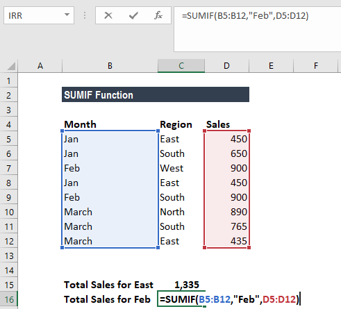
Suppose we are given the following data:

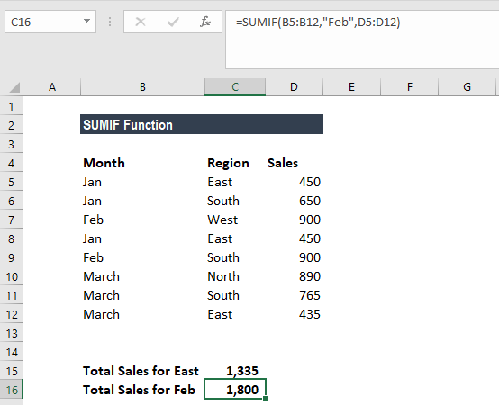
We wish to find total sales for the East region and the total sales for February. The formula to use to get the total sales for East is:

SUMIF Function - Example 1

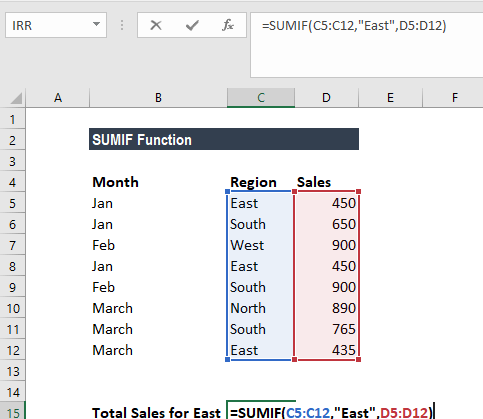
Text criteria, or criteria that includes math symbols, must be enclosed in double quotation marks (” “).

We get the result below:

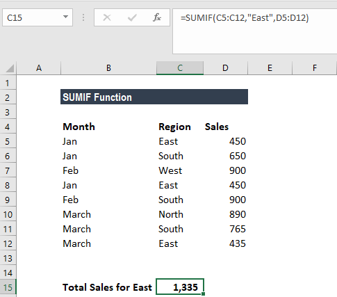
The formula for total sales in February is:

We get the result below:

A few notes about the SUMIF Excel Function

#VALUE! error – Occurs when the criteria provided is a text string that is more than 255 characters long.
When sum_range is omitted, the cells in range will be summed.
The following wildcards can be used in text-related criteria:
- ? – matches any single character
- * – matches any sequence of characters
To find a literal question mark or asterisk, use a tilde (

) in front of the question mark or asterisk (i.e.

Additional resources

Thanks for reading CFI’s guide to important Excel functions! By taking the time to learn and master these functions, you’ll significantly speed up your financial analysis. To learn more, check out these additional CFI resources:

Excel Functions for Finance Excel for Finance This Excel for Finance guide will teach the top 10 formulas and functions you must know to be a great financial analyst in Excel.
Advanced Excel Formulas You Must Know Advanced Excel Formulas Must Know These advanced Excel formulas are critical to know and will take your financial analysis skills to the next level. Download our free Excel ebook!
Excel Shortcuts for PC and Mac Excel Shortcuts PC Mac Excel Shortcuts — List of the most important & common MS Excel shortcuts for PC & Mac users, finance, accounting professions. Keyboard shortcuts speed up your modeling skills and save time. Learn editing, formatting, navigation, ribbon, paste special, data manipulation, formula and cell editing, and other shortucts

Интересно почитать: Если функции эксель

Free Excel Tutorial

To master the art of Excel, check out CFI’s FREE Excel Crash Course, which teaches you how to become an Excel power user. Learn the most important formulas, functions, and shortcuts to become confident in your financial analysis.

SUMIF Excel Function

The SUMIF Excel function calculates the sum of a range of cells based on given criteria. The criteria can include dates, numbers, and text. For example, the formula “=SUMIF(B1:B5, “<=12”)” adds the values in the cell range B1:B5, which are less than or equal to 12.

SUMIF function is categorized under the Excel Math and Trigonometry functions. Moreover, this function works similar to the SUMIFS function SUMIFS Function In Excel, SUMIFS is an in-built function that calculates the sum of all those cells which meet the multiple specified criteria & it is widely used as a conditional statement. read more . The SUMIF function uses a single criterion, whereas the SUMIFS function uses multiple criteria.

SUMIF Formula in Excel

The SUMIF formula is stated as follows:

The formula accepts the following arguments:

Range: It refers to the range of cells on which the criteria is applied.
Criteria: It refers to the conditions that are applied to the range of cells. It determines the cells to be added from the given “sum_range.”
Sum_range: It indicates the range of cells to be added together.

“Range” and “criteria” are the required parameters, whereas “sum_range” is an optional parameter.

Note: If “sum_range” is not specified, the SUMIF function refers to the parameter “range” as the range of cells to be added.

How to Use the SUMIF Excel Function?

Let us understand the SUMIF excel function with the help of the following examples. Each example covers a different case, implemented using the SUMIF function.

Example #1

Total Amount Spent on Branded Televisions (TVs)

The following table shows a list of branded equipment and their prices. For some equipment, the brands are not specified. We have to calculate the total amount spent on purchasing branded TVs using the SUMIF function.

In the succeeding table, the cells that satisfy the given criteria are C4, C7, and C10, which shows the prices of the branded TVs. Hence, the sum of the values of cells C4, C7, and C10 is 1,73,000, shown in cell C14. This is the total amount spent on purchasing branded TVs.

The following SUMIF formula is applied to the range C2:C11:

B2:B11 refers to the range of cells on which the specific criterion is to be applied.
“TV” refers to the condition applied to the range B2:B11.
C2:C11 refers to the range of values to be added.

Example #2

Sum of the Amount Spent on Non-Branded Items

Working on the data of example #1, we want to calculate the total amount spent on purchasing non-branded items using the SUMIF function.

In the following table, the cells C11 and C12 satisfy the given criteria where no brand name is entered in the cells. Hence, the sum of the values of cells C11and C12 is 53,000, as shown in cell C14. This indicates the total amount spent on purchasing non-branded items.

The following SUMIF formula is applied to the range C2:C12:

A2:A12 refers to the range of cells on which the specific criterion is to be applied.
“” refers to the condition which checks for blank cells in the range B2:B12.
C2:C12 is the range of values to be summed up.

Example #3

Sum of the Amount Spent on Branded Items

Working on the data of example #1, we want to calculate the total amount spent on branded items using the SUMIF function.

Интересно почитать: Функция промежуточные итоги в excel

In the following table, the cells B11, B12 satisfy the given criteria with no brand names. Hence, the sum of the values of C1 to C10 is 53,000, displayed in cell C14. This is the total amount spent on purchasing branded items. The cells C11 and C12 are skipped because they are blank cells.

The following SUMIF formula is applied to the range C2:C12:

A2:A12 refers to the range on which the criteria are to be applied.
“<>” is the condition which checks for non-blank cells in the range B2:B12.
C2:C12 is the range of values to be added.

Example #4

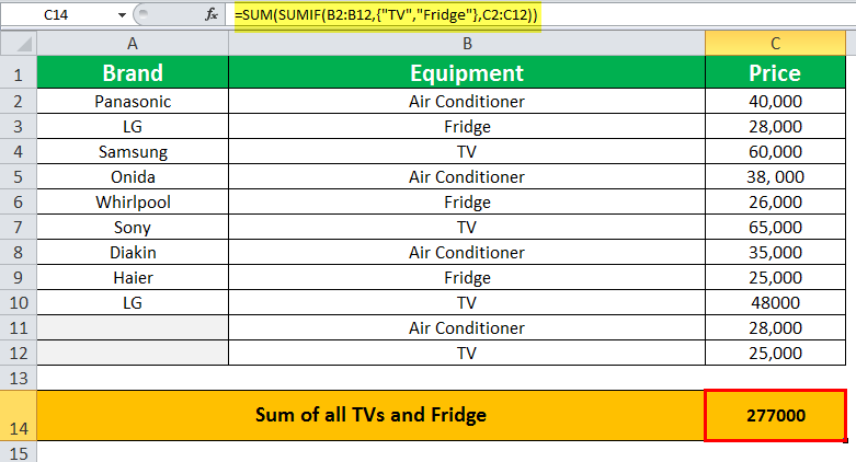
Sum of the Two Different Items

Working on the data of example #1, we want to calculate the sum of two different items using the SUMIF formula.

The following table shows the total amount calculated by adding the sum of the prices of two items – TV and fridge in the cell C14, using the SUMIF formula. The SUM of the prices of the fridges and TVs are 79,000 and 1,98,000, respectively. Hence, the total SUM of the prices of two items is 2,77,000.

The SUMIF formula is applied to the range C2:C12 and is stated as follows:

B2: B12 refers to the range on which the criteria are to be applied.
“TV,” “fridge” refers to the two individual conditions to be checked in range B2: B12. The curly braces <> of the criterion represent the collection of constants.
C2: C12 refers to the range of values to be added.

The “Criteria” Argument of the SUMIF Function

The guidelines of the argument of the SUMIF formula are stated as follows:

The numeric criteria are not enclosed in double quotes.
The text criteria for SUMIFText Criteria For SUMIFSUMIF function is a conditional IF function to sum the cells based on specific criteria. For example, to add a group of cells, if the cell adjacent to them has a specified text in them, then function is used as follows =SUMIF(Text Range,” Text”, cells range for sum).read more , including the mathematical symbols, are enclosed within double quotes.
The wildcard characters – question mark (?) and asterisk (*) used in the criteria match a single character and a series of characters, respectively.
The tilde operator (

) followed by the wildcard characters refer to the actual characters. For example, the “

Frequently Asked Questions (FAQs)

The SUMIF function returns the sum of cells that satisfy the given criteria. This worksheet (WS) function is categorized as a Math and Trigonometry function. Furthermore, for partial matching, it uses logical operators and wildcards.

The SUMIF formula is stated as follows:
“=SUMIF(range, criteria, [sum_range])”
Where,

• Range refers to the range of cells against which we need to apply the criteria.
• Criteria are the conditions that are applied to the range of cells.
• Sum_range is an array of numeric values. The values are added if the specific criterion matches the range.

The “range” and “criteria” are the required arguments, and “sum_range” is an optional argument.

Note: If the argument “sum_range” is omitted, the values in the “range” will be added.

The formula for the SUMIF with multiple criteria is stated as follows:
“=SUMIF(sum_range, range 1, criteria1)+SUMIF(sum_range, range 2, criteria2)”

Where,
• Sum_range refers to the range of cells to be added.
• Range1, range 2 are the range of cells on which the criteria are to be applied.
• Criteria1, criteria 2 are the conditions applied to the respective range of cells. Alternatively, we can use the SUMIFS function to sum cells satisfying the multiple criteria.

The SUMIF excel function can be used to add cells containing text strings that meet specific criteria. In the formula, the text criteria are enclosed in double quotes.

For example, consider the below SUMIF formula:
“=SUMIF(A1:A4,“Purple”,B1:B4)”

The formula adds the values in range B1:B4 if the range A1:A4 contains the text “Purple”.