RANK Function Examples In Excel, VBA,; Гугл Sheets

RANK Function Examples In Excel, VBA, & Гугл Sheets

This tutorial demonstrates how to use the Excel RANK Function in Excel to rank a number within a series.

RANK Function Overview

The RANK Function Rank of a number within a series.

To use the RANK Excel Worksheet Function, select a cell and type:

(Notice how the formula inputs appear)

RANK function Syntax and inputs:

number – The number that you wish to determine the rank of.

ref – An array of numbers.

order – OPTIONAL. A number indicating whether to rank descendingly (0 or Ommitted) or ascendingly (non-zero number)

What Is the RANK Function?

The Excel RANK Function tells you the rank of a particular value taken from a data range. That is, how far the value is from the top, or the bottom, when the data is put into order.

RANK Is a “Compatibility” Function

As of Excel 2010, Microsoft replaced RANK with two variations: RANK.EQ and RANK.AVG.

The older RANK Function still works, so any older spreadsheets using it will continue to function. However, you should use one of the newer functions whenever you don’t need to remain compatible with older spreadsheets.

How to Use the RANK Function

Use RANK like this:

Above is a table of data listing the heights of a group of friends. We want to know where Gunther ranks in the list.

RANK takes three arguments:

• The first is the value you want to rank (we’ve set this to C10, Gunther’s height, but we could also put the value in directly as 180)
• The second is range of data – C4:C13
• The third is the order of the rank
  • If you set this to FALSE, 0, or leave it blank, the highest value will be ranked as #1 (descending order)
  • If you set this to TRUE or any non-zero number, the lowest value will be ranked as #1 (ascending order)

  RANK determines that Gunther is the 4 th tallest of the group, and if we put the data in order, we see that this is true:

  A few key points about the RANK Function:

  • When determining the order, text strings will result in a #VALUE! error
  • As you’ve just seen, you don’t need to sort the data for RANK to work correctly

  How RANK Handles Ties

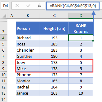
  In the below table I’ve added a column to the table that returns the rank of each member of the group. I used the following formula:

  Note that I’ve locked the data range $C$4:$C$13 by select “C4:C13” in the formula bar, and then pressing F4. This keeps this part of the formula the same so that you can copy it down the table without it changing.

  

  We have a tie! Both Joey and Mike are 178cm tall.

  In such cases, RANK assigns both values the highest rank – so both Joey and Mike are ranked 5 th . Because of the tie, there is no 6 th place, so the next tallest friend, Phoebe, is in 7 th place.

  How to Use RANK.EQ

  RANK.EQ works in the same way as RANK. You use it like this:

  

  As you can see here, with RANK.EQ you define exactly the same arguments as with RANK, namely, the number you want to rank, the data range, and the order. We’re looking for Gunther’s rank again, and RANK.EQ returns the same result: 4.

  RANK.EQ also handles ties in the same way as RANK, as shown below:

  

  Again, Joey and Mike are tied at 5th place.

  How to Use RANK.AVG

  RANK.AVG is very similar to RANK.EQ and RANK. It only differs in the way it handles ties. So if you’re just looking for the rank of a single value, all three functions will return the same result:

  

  Once again, the same result – 4 th place for Gunther.

  Now let’s look at how RANK.AVG differs in terms of ties. So this time I’ve used this function:

  And here are the results:

  

  Now we see something different!

  RANK.AVG gives Joey and Mike the same rank, but this time they are assigned the average rank that they would have received had their heights not been equal.

  So, they would have been ranked 5 th and 6 th , but RANK.AVG has returned the average of 5 and 6: 5.5.

  If more than two values are tied, the same logic applies. Let’s pretend Phoebe has a sudden growth spurt, and her height increases to 178cm overnight. Now RANK.AVG returns the following:

  

  All three friends how rank 6 th : (5 + 6 + 7) / 3 = 6.

  RANK IF Formula

  Excel doesn’t have a built-in formula that enables you to rank values based on a given criteria, but you can achieve the same result with COUNTIFS.

  Say the friends want to create two separate rank orders, one for males and one for females.

  Here’s the formula we’d use:

  

  COUNTIFS counts the number of values in a given data range that meet criteria you specify. The formula looks a little intimidating, but it makes more sense if we break it down line-by-line:

  So the first criteria we’ve set is that the range in C4:C13 (again, locked with the dollar signs so that we can drag the formula down the table without that range changing) must match the value in C4.

  So for this row, we’re looking at Richard, and his value is C4 is “Male”. So we’re only going to count people who also have “Male” in this column.

  The second criteria is that D4:D13 must be higher than D4. Effectively, this returns the number of people in the table who’s value in the D column is greater than Richard’s.

  Then we add 1 to the result. We need to do this because no one is taller than Richard, so the formula would return 0 otherwise.

  Conditional Ranking in Excel using SUMPRODUCT Function [RANKIF]

  First of all just do this for me, open your Excel workbook and try to type RANKIF.

  You will be wondered that there is no function in Excel for conditional ranking.

  Yes, there is no one.

  Now, just think this way, have you ever faced a situation where you have to rank values by using some specific criteria?

  And if yes, then how you solved that problem, because you know there is no RANKIF function in Excel.

  Let me tell you something, whenever you want to create a conditional ranking based on a specific criterion or category wise ranking, the best way is to use SUMPRODUCT.

  Yes, you get it right, it’s SUMPRODUCT.

  I’m in love with this function from the last couple of years and today, in this post I will show you a simple way to rank values with a condition by using SUMPRODUCT.

  A simple way, no big deal. And, this is a kind of technique which can drive you from beginner to advanced Excel user.

  …so, let’s get started.

  Here in this example, we have a list of students with their score in different subjects. You can download this sample file from here to follow along.

  

  Here our target is to rank all the students in each of the subjects. That means, ranking from first to the last student in each subject like Finance, Operations and so on, according to their marks

  Conditional Formula to use as RANKIF

  • First of all, add a new column at the end of the table and name it “Subject Wise Rank”.
    
  • in the D4 cell, enter this formula =SUMPRODUCT((–(C2=$C$2:$C$121)),(–(B2<$B$2:$B$121)))+1 and hit enter.
    
  • After that, apply that formula to the end of the column, up to the last cell.
    

  Congratulations , you have added subject wise ranks for the students, and do you believe you took a few seconds.

  Isn’t it simple and effective?

  But, the important part is to understand that how this formula works.

  And believe me, you’ll be surprised when you get to know that you have done a magic here with this function.

  How this Conditional RANKIF Formula works

  To understand this we need to break this formula into three parts.

  And, please remember SUMPRODUCT is a function which can take arrays even when you haven’t applied a formula as an array.

  Part-1: Compare Names

  In the first part, you have used (–(C2=$C$2:$C$121)) to compare a subject name with the entire range.

  And, it will return an array in which all those values will be true which are matched with the subject name “Finance”.

  To check, just edit your formulas in cell D4, select only first part of the formula and press F9. It will show all the values of the array.

  Here all the values which are matched with the subject name from the cell D4 are TRUE and the others are FALSE.

  So the point is, it has returned a TRUE in the entire array where the subject name is matched.

  And in the end, you have to use the double minus sign to convert TRUE and FALSE into 1 and 0.

  Part-2: Check Greater than Values

  In the second part, you have used (–(B2<$B$2:$B$121)) to check other student’s score which is greater than the Tameka’s score.

  And, it returns an array in which all the values are TRUE where marks are greater than Tameka.

  To check, just edit your formulas in cell D4, select only second part of the formula and press F9. It will show all the values of the array.

  Here all the values which are greater than “24” are TRUE and others are FALSE.

  So the point is, it has returned a TRUE in the entire array where the scores are greater than “24”.

  And in the end, you have to use the double minus sign to convert TRUE and FALSE into 1 and 0. Now, it will look like this.

  Part-3: Multiply Two Arrays

  Now take a deep breath and relax. Slow down your mind and think like this. At this point, we have two different arrays.

  1. In the first array, you have 1 for all values where the subject is matched and 0 if not matched.
  2. In the second array, you have 1 for all the values where the score of the students are greater and 0 if equal or lower.

  Now, when SUMPRODUCT multiplies these two arrays you will get 1 only for those students whose subject is matched and the score is greater than Tameka.

  Just look at this, there are 9 other students with greater than marks from Tameka in Finance.

  Part-4: Adding + ONE

  If you are curious to know about why you need to add 1 in the final formula then here is the reason for this:

  At this point, you know that a total of 9 students is there whose marks are greater than Tameka. So, if 9 students are there then Tameka should be on 10th rank.

  That’s why you need to add 1 at the end of the formula.

  Sample File

  Conclusion

  If you ask me, I believe SUMPRODUCT is one of the most powerful functions in Excel library and the method we have used above is simple and effective.

  With SUMPRODUCT, you don’t need to write long nesting conditional formulas. You just need this magic trick to add conditional ranks.

  I hope this tip will help you in your work and now, tell me one thing.

  Do you know any other method to creating RANKIF?

  Please share your views with me in the comment section, I’d love to hear from you and please don’t forget to share this tip with your friends.

  Создаем генератор случайных чисел в Excel

  Хорошего времени суток, почетаемый, читатель!

  Не так давно, появилась необходимость сделать типичный генератор случайных чисел в Excel в границах подходящей задачки, а она была обычная, с учётом количества человек избрать случайного юзера, всё весьма просто и даже обыденно. Но меня заинтриговало, а что все-таки ещё можно созодать при помощи такового генератора, какие они бывают, каковые их функции для этого употребляются и в каком виде. Вопросцем много, так что равномерно буду и отвечать на их.

  Итак, для чего же же фактически мы можем применять этом механизм:

  • во-1-х: мы можем для тестировки формул, заполнить подходящий нам спектр случайными числами;
  • во-2-х: для формирования вопросцев разных тестов;
  • в-третьих: для хоть какого случаем распределения заблаговременно пронумерованных задач меж вашими сотрудниками;
  • в-четвёртых: для симуляции разнообразнейших действий;

  …… ну и в почти всех остальных ситуациях!

  В данной для нас статье я рассмотрю лишь 3 варианта сотворения генератора (способности макроса, я не буду обрисовывать), а конкретно:

  1. При помощи функции СЛЧИС;
  2. При помощи функции СЛУЧМЕЖДУ;
  3. При помощи надстройки AnalysisToolPack.

  Создаём генератор случайных чисел при помощи функции СЛЧИС
  

  При помощи функции СЛЧИС, мы имеем возможность генерировать хоть какое случайное число в спектре от 0 до 1 и эта функция будет смотреться так:

  

  Если возникает необходимость, а она, быстрее всего, возникает, применять случайное число огромного значения, вы просто сможете помножить вашу функцию на хоть какое число, например 100, и получите:

  

  =СЛЧИС()*100; А вот если для вас не нравятся дробные числа либо просто необходимо применять целые числа, тогда используйте такую комбинацию функций, это дозволит для вас отсечь значения опосля запятой либо просто откинуть их:

  

  =ОТБР((СЛЧИС()*100);0) Когда возникает необходимость применять генератор случайных чисел в каком-то определённом, определенном спектре, согласно нашим условиям, например, от 1 до 6 нужно применять последующую систему (непременно закрепите ячейки при помощи абсолютных ссылок):

  • a – представляет нижнюю границу,
  • b – верхний предел

  и полная формула будет смотреться: =СЛЧИС()*(6-1)+1, а без дробных частей для вас необходимо написать: =ОТБР(СЛЧИС()*(6-1)+1;0)

  

  Создаём генератор случайных чисел при помощи функции СЛУЧМЕЖДУ
  

  Эта функция наиболее ординарна и начала нас веселить в базисной комплектации Excel, опосля 2007 версии, что существенно облегчило работу с генератором, когда нужно применять спектр. Например, для генерации случайного числа в спектре от 20 до 50 мы будем применять систему последующего вида:

  

  Создаём генератор при помощи надстройки AnalysisToolPack
  

  В 3-ем методе не употребляется никакая функция генерации, а всё делается при помощи надстройки AnalysisToolPack (эта надстройка заходит в состав Excel). Интегрированный в табличном редакторе инструмент можно применять как инструмент генерации, но необходимо знать если вы желаете поменять набор случайных чисел, то для вас необходимо эту функцию перезапустить.

  Для получения доступа к данной для нас, безусловн, полезной надстройки, необходимо, для начала, при помощи диалогового окна «Надстройки» установить этот пакет. Если у вас он уже установлен, то дело за малым, выбираете пункт меню «Данные» – «Анализ» – «Анализ данных», выбираете «Генерация случайных чисел» в предложенном программкой перечне и жмём «ОК».

  

  В открывшемся окне мы избираем тип в меню «Распределение», опосля указываем доп характеристики, которые меняются, исходя с типа распределения. Ну и финишный шаг, это указание «Выходной интервал», конкретно тот интервал где будут храниться, ваши случайные числа.

  

  А на этом у меня всё! Я весьма надеюсь, что вопросец по созданию генератора случайных чисел я раскрыл стопроцентно и для вас всё понятно. Буду весьма признателен за оставленные комменты, потому что это показатель читаемости и побуждает на написание новейших статей! Делитесь с друзьями прочитанным и ставьте лайк!

  Не забудьте поблагодарить создателя!

  Не додумывай очень много. Так ты создаешь препядствия, которых вначале не было.

  RANK Function

  The RANK Function is categorized as an Excel Statistical function Functions List of the most important Excel functions for financial analysts. This cheat sheet covers 100s of functions that are critical to know as an Excel analyst . The function returns the statistical rank of a given value within a supplied array of values. Thus, it determines the position of a specific value in an array.

  Formula

  =RANK(number,ref,[order])

  The RANK function uses the following arguments:

  1. Number (required argument) – This is the value for which we need to find the rank.
  2. Ref (required argument) – Can be a list of, or an array of, or reference to, numbers.
  3. Order (optional argument) – This is a number that specifies how the ranking will be done (ascending or descending order).
     • 0 – is used for descending order
     • 1 – is used for ascending order
     • If we omit the argument, it will take a default value of 0 (descending order). It will take any non-zero value as the value 1 (ascending order).

  Before we proceed, we need to know that the RANK function has been replaced by RANK.EQ and RANK.AVG. To enable backward compatibility, RANK still works in Excel 2016 (latest version), but it may not be available in the future. If you type this function in Excel 2016, it will show a yellow triangle with an exclamation point.

  How to use the RANK Function in Excel?

  As a worksheet function, RANK can be entered as part of a formula in a cell of a worksheet. To understand the uses of the function, let’s consider a few examples:

  Example 1

  Assume we are given a list of employees with their respective medical reimbursement expenses. We wish to rank them according to total expenditure.

  

  To rank in descending order, we will use the formula =RANK(B2,($C$5:$C$10),0), as shown below:

  The result we get is shown below:

  

  As seen above, the RANK function gives duplicate numbers the same rank. However, the presence of duplicate numbers affects the ranks of subsequent numbers. For example, as shown above, in a list of integers sorted in ascending order, the number 100 appears twice with a rank of 4. The next value (25) will be ranked 6 (no number will be ranked 5).

  If we want unique ranks, we can use the formula:

  =RANK(C5,$C$5:C$10,0)+COUNTIF($C$5:C5,C5)-1

  

  We will get the results below:

  

  For ascending order, the formula would be:

  =RANK.EQ(C5,$C$5:C$10,1)+COUNTIF($C$5:C5,C5)-1

  In both formulas, it’s the COUNTIF function that does the trick. We used COUNTIF to find out the number of times the ranked number occurred. In the COUNTIF formula, the range consists of a single cell ($C$5:C5). As we locked only the first reference ($C$5), the last relative reference (C5) changes based on the row where the formula is copied. Thus, for row 7, the range expands to $C$5:C10, and the value in C10 is compared to each of the above cells.

  Thus, for all unique values and first occurrences of duplicate values, COUNTIF returns 1; and we subtract 1 at the end of the formula to restore the original rank.

  For ranks occurring the second time, COUNTIF returns 2. By subtracting 1, we increased the rank by 1 point, thus preventing duplicates. If there happen to be 3+ occurrences of the same value, COUNTIF()-1 would add 2 to their ranking, and so on.

  Things to remember about the RANK Function

  1. #N/A! error – Occurs when the given number is not present in the supplied reference. Also, the RANK function does not recognize text representations of numbers as numeric values, so we will also get the #N/A error if the values in the supplied ref array are text values.
  2. If we provide logical values, we will get the #VALUE! error.

  Additional resources

  Thanks for reading CFI’s guide to important Excel functions! By taking the time to learn and master these functions, you’ll significantly speed up your financial analysis. To learn more, check out these additional CFI resources:

  • Excel Functions for Finance Excel for Finance This Excel for Finance guide will teach the top 10 formulas and functions you must know to be a great financial analyst in Excel.
  • Advanced Excel Formulas You Must Know Advanced Excel Formulas Must Know These advanced Excel formulas are critical to know and will take your financial analysis skills to the next level. Download our free Excel ebook!
  • Excel Shortcuts for PC and Mac Excel Shortcuts PC Mac Excel Shortcuts — List of the most important & common MS Excel shortcuts for PC & Mac users, finance, accounting professions. Keyboard shortcuts speed up your modeling skills and save time. Learn editing, formatting, navigation, ribbon, paste special, data manipulation, formula and cell editing, and other shortucts

  Free Excel Tutorial

  To master the art of Excel, check out CFI’s FREE Excel Crash Course, which teaches you how to become an Excel power user. Learn the most important formulas, functions, and shortcuts to become confident in your financial analysis.

  Интересно почитать:  Формула в excel если значение меньше 0 то равно 0