Index Match Formula

The INDEX MATCH formula is the combination of two functions in Excel Excel Resources Learn Excel online with 100’s of free Excel tutorials, resources, guides & cheat sheets! CFI’s resources are the best way to learn Excel on your own terms. : INDEX and MATCH.

=INDEX() returns the value of a cell in a table based on the column and row number.

=MATCH() returns the position of a cell in a row or column.

Combined, the two formulas can look up and return the value of a cell in a table based on vertical and horizontal criteria. For short, this is referred to as just the Index Match function. To see a video tutorial, check out our free Excel Crash Course.

#1 How to Use the INDEX Formula

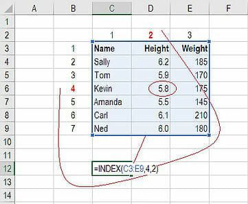
Below is a table showing people’s names, height, and weight. We want to use the INDEX formula to look up Kevin’s height… here is an example of how to do it.

Follow these steps:

1. Type “=INDEX(” and select the area of the table, then add a comma
2. Type the row number for Kevin, which is “4,” and add a comma
3. Type the column number for Height, which is “2,” and close the bracket
4. The result is “5.8.”

#2 How to Use the MATCH Formula

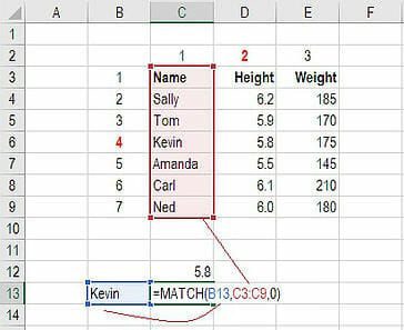
Sticking with the same example as above, let’s use MATCH to figure out what row Kevin is in.

Follow these steps:

1. Type “=MATCH(” and link to the cell containing “Kevin”… the name we want to look up.
2. Select all the cells in the Name column (including the “Name” header).
3. Type zero “0” for an exact match.
4. The result is that Kevin is in row “4.”

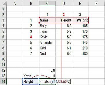
Use MATCH again to figure out what column Height is in.

Follow these steps:

1. Type “=MATCH(” and link to the cell containing “Height”… the criteria we want to look up.
2. Select all the cells across the top row of the table.
3. Type zero “0” for an exact match.
4. The result is that Height is in column “2.”

#3 How to Combine INDEX and MATCH

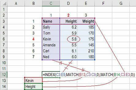
Now we can take the two MATCH formulas and use them to replace the “4” and the “2” in the original INDEX formula. The result is an INDEX MATCH formula.

Follow these steps:

1. Cut the MATCH formula for Kevin and replace the “4” with it.
2. Cut the MATCH formula for Height and replace the “2” with it.
3. The result is Kevin’s Height is “5.8.”
4. Congratulations, you now have a dynamic INDEX MATCH formula!

Video Explanation of How to Use Index Match in Excel

Below is a short video tutorial on how to combine the two functions and effectively use Index Match in Excel! Check out more free Excel tutorials on CFI’s YouTube Channel.

Hopefully, this short video мейд it even clearer how to use the two functions to dramatically improve your lookup capabilities in Excel.

More Excel Lessons

Thank you for reading this step-by-step guide to using INDEX MATCH in Excel. To continue learning and advancing your skills, these additional CFI resources will be helpful:

• Excel Formulas and Functions List Functions List of the most important Excel functions for financial analysts. This cheat sheet covers 100s of functions that are critical to know as an Excel analyst
• Excel Shortcuts Excel Shortcuts PC Mac Excel Shortcuts — List of the most important & common MS Excel shortcuts for PC & Mac users, finance, accounting professions. Keyboard shortcuts speed up your modeling skills and save time. Learn editing, formatting, navigation, ribbon, paste special, data manipulation, formula and cell editing, and other shortucts
• Go To Special Go To Special Go To Special in Excel is an important function for financial modeling spreadsheets. The F5 key opens Go To, select Special Shortcuts for Excel formulas, allowing you to quickly select all cells that meet certain criteria.
• Find and Replace Find and Replace in Excel Learn how to search in Excel — this step by step tutorial will teach how to Find and Replace in Excel spreadsheets using Ctrl + F shortcut. Excel find and replace allows you to quickly search all cells and formulas in a spreadsheet for all instances that match your search criteria. This guide will cover how to
• IF AND F IF Statement Between Two Numbers Download this free template for an IF statement between two numbers in Excel. In this tutorial, we show you step-by-step how to calculate IF with AND statement.
• unction in Excel IF Statement Between Two Numbers Download this free template for an IF statement between two numbers in Excel. In this tutorial, we show you step-by-step how to calculate IF with AND statement.

Free Excel Tutorial

To master the art of Excel, check out CFI’s FREE Excel Crash Course, which teaches you how to become an Excel power user. Learn the most important formulas, functions, and shortcuts to become confident in your financial analysis.

MS Excel: How to use the MATCH Function (WS)

This Excel tutorial explains how to use the Excel MATCH function with syntax and examples.

Description

The Microsoft Excel MATCH function searches for a value in an array and returns the relative position of that item.

The MATCH function is a built-in function in Excel that is categorized as a Lookup/Reference Function. It can be used as a worksheet function (WS) in Excel. As a worksheet function, the MATCH function can be entered as part of a formula in a cell of a worksheet.

If you want to follow along with this tutorial, download the example spreadsheet.

Syntax

The syntax for the MATCH function in Microsoft Excel is:

Parameters or Arguments

Optional. It the type of match that the function will perform. The possible values are:

If the match_type parameter is omitted, it assumes a match_type of 1.

Returns

The MATCH function returns a numeric value.
If the MATCH function does not find a match, it will return a #N/A error.

The MATCH function does not distinguish between upper and lowercase when searching for a match.

If the match_type parameter is 0 and the value is a text value, then you can use wildcards in the value parameter.

Applies To

• Excel for Office 365, Excel 2019, Excel 2016, Excel 2013, Excel 2011 for Mac, Excel 2010, Excel 2007, Excel 2003, Excel XP, Excel 2000

Type of Function

• Worksheet function (WS)

Example (as Worksheet Function)

Let’s look at some Excel MATCH function examples and explore how to use the MATCH function as a worksheet function in Microsoft Excel:

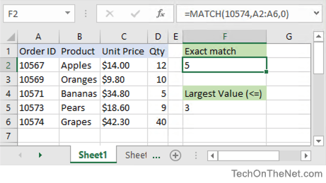
Based on the Excel spreadsheet above, the following MATCH examples would return:

Let’s look at how we can use wild cards in the MATCH function.

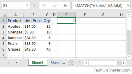
Based on the Excel spreadsheet above, the following MATCH examples would return:

Frequently Asked Questions

Question: In Microsoft Excel, I tried this MATCH formula but it did not work:

I was hoping for an easier formula than this:

Answer: When you are using the MATCH function, you need to be aware of a few things.

First, you need to consider whether your array is sorted in a particular order (ie: ascending order, descending order, or no order). Since we are looking for an exact match and we don’t know if the array is sorted, we want to make sure that the match_type parameter in the MATCH function is set to 0. This will find a match regardless of the sort order.

Second, we know that the MATCH function will return an #N/A error when a match is not found, so we will want to use the ISERROR function to check for the #N/A error.

So based on these 2 additional considerations, we would want to modify your original formula as follows:

This would check for an exact match in the D54:D96 array on the Overview sheet and return «FS» if a match is found. Otherwise, it would return «Bulk» if no match is found.

Question: I have a question about how to nest a MATCH function within the INDEX function. The question is:

I want to create a formula using the MATCH function nested within the INDEX function to retrieve the Class that was selected (by the x) in E4:F10. The MATCH function should find the row where the x is located and should be used within the INDEX function to retrieve the associated Class value from the same row within F4:F10.

Answer: We can use the MATCH function to find the row position in the range E4:E10 to find the row where "x" is located. We then embed this MATCH function within the INDEX function to return the corresponding value in the range F4:$10 as follow:

In this example, we are searching for the value "x" within the range E4:E10. When the value of "x" is found, it will return the corresponding value from F4:F10.

Функцията MATCH в Microsoft Excel

Един от най-популярните оператори сред потребителите на Excel е функцията MATCHING . Неговата задачка е да обусловь номера на елемента в даден набор от данни. Най-голямата полза, която носи, когато се използва съвместно с други оператори. Да лицезреем каква е функцията на MATCH и как може да се използва на практика.

Използване на оператора MAP

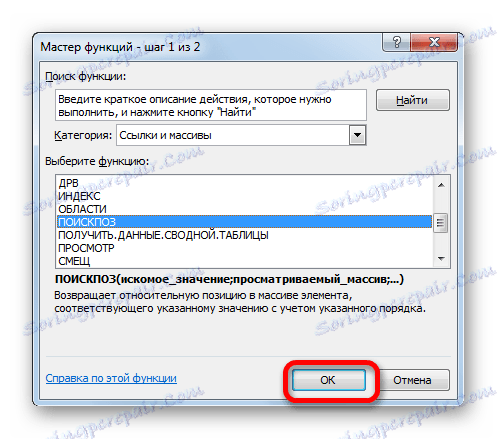
Операторът на MAP принадлежи към категорията "Връзки и масиви" . Той търси определения елемент в посочения масив и връща номера на своята позиция в този спектр на отделна клеточка. Всъщност дори името му показва това. Също така, когато се комбинира с други оператори, тази функция ги информира за номера на позицията на даден елемент за последваща обработка на тези данни.

Синтаксисът на израза MATCH изглежда така:

Сега разгледайте всеки от тези три аргумента отделно.

"Търсенето на смисъл" е елементът, който трябва да се намери. Тя може да има текстова, цифрова форма и да има логическа стойност. Този аргумент може да бъде и препратка към клеточка, която съдържа някоя от горепосочените стойности.

"Сканираният масив" е адресът на спектра, в който се намира стойността. Позицията на този елемент в този масив трябва да бъде определена от оператора на MAP .

"Тип на съвпадението " показва точното съвпадение, което искате да търсите либо неточно. Този аргумент може да има три стойности: "1" , "0" и "-1" . Ако стойността е "0", операторът търси само буквально съвпадение. Ако стойността "1" е посочена, при отсъствието на буквально съвпадение MATCH произвежда най-близкия елемент към нея в низходящ ред. Ако стойността е "-1" , тогава в варианта, ако точното съвпадение не е хочет, функцията произвежда най-близкия елемент към него във възходящ ред. Принципиально е, ако търсенето не е точна, но приблизителна, така че масива, който ще се сканира, се подрежда във възходящ ред (тип на картографиране "1" ) либо низходящ (тип на картографиране "-1" ).

Аргументът "Съответстващ тип" е по избор. Това може да се пропусне, ако не е нужно. В този вариант стойността му по подразбиране е "1" . Прилагането на аргумента "Тип на съвпадението" има преди всичко смисъл само когато се обработват цифрови стойности, а не текст.

Ако MATCH за определените опции не може да намери желания елемент, операторът показва грешката "# N / D" в клетката.

При извършване на търсене операторът не прави разлика меж регистрите на знаци. Ако има няколко точни съвпадения в масива, тогава MATCHING показва позицията на първия в клетката.

Способ 1: Показване на мястото на елемент в спектр от текстови данни

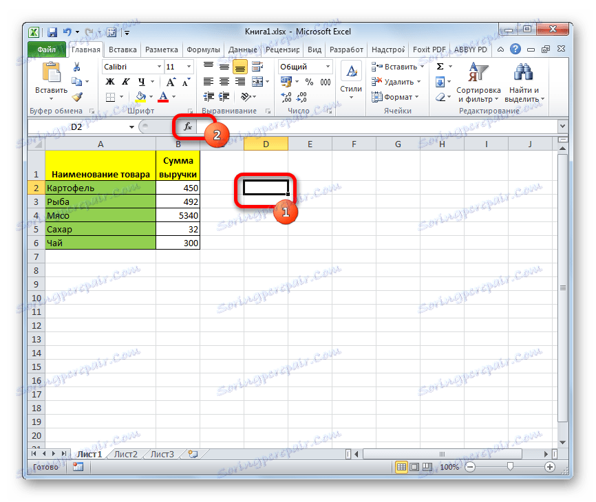
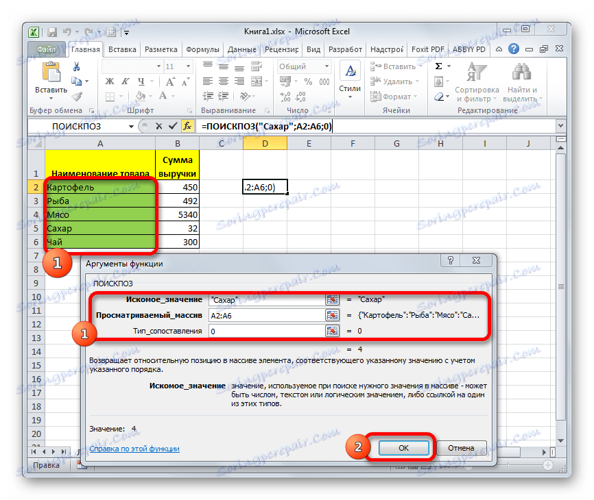
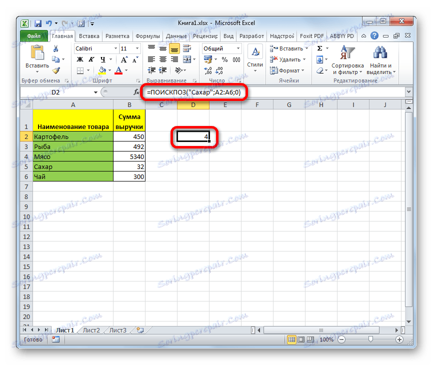
Нека да разгледаме примера на най-простия вариант, когато използвате MATCH, сможете да обусловьте местоположението на посочения елемент в масив от текстови данни. Ще открием коя позиция в обхвата, в който се намират имената на стоките, е думата "захар" .

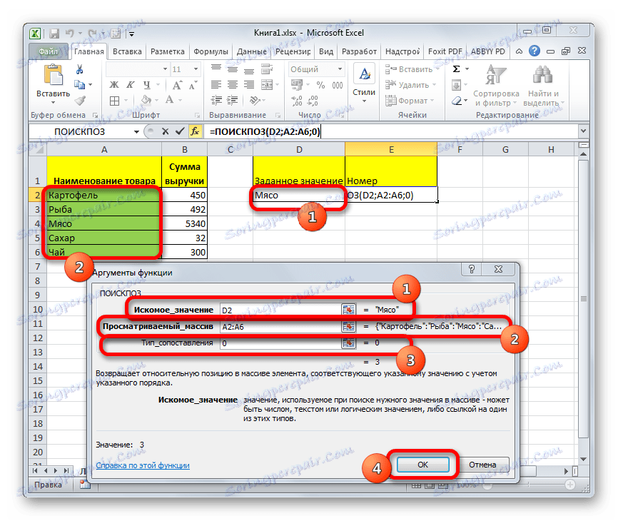
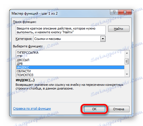
Изберете клетката, в която ще се извежда обработеният резултат. Кликнете върху иконата "Вмъкване на функция" до лентата за формули.

Тъй като трябва да намерим позицията на думата "Sugar" в спектра, караме това име в полето "Search value" .

В полето "Сканиран масив" трябва да посочите координатите на самия спектр. Той може да бъде изкован ръчно, но е по-лесно да поставите курсора в полето и да изберете този масив на листа, като задържите левия бутон на мишката. След това адресът му ще се покаже в прозореца с аргументи.

В третото поле "Съответстващ тип" поставяме числото "0" , тъй като ще работим с текстови данни и затова се нуждаем от точен резултат.

Способ 2: Автоматизиране на използването на оператора MATCH

По-горе разгледахме най-примитивния вариант на използване на POSITION оператора, но дори и той може да бъде автоматизиран.

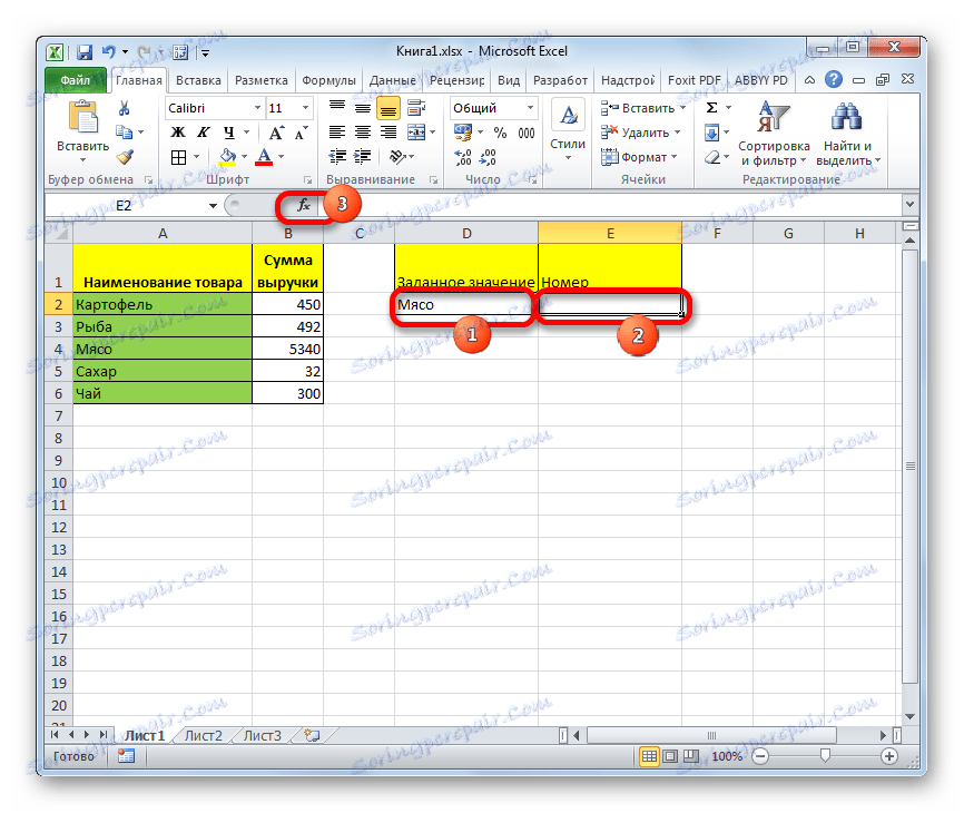
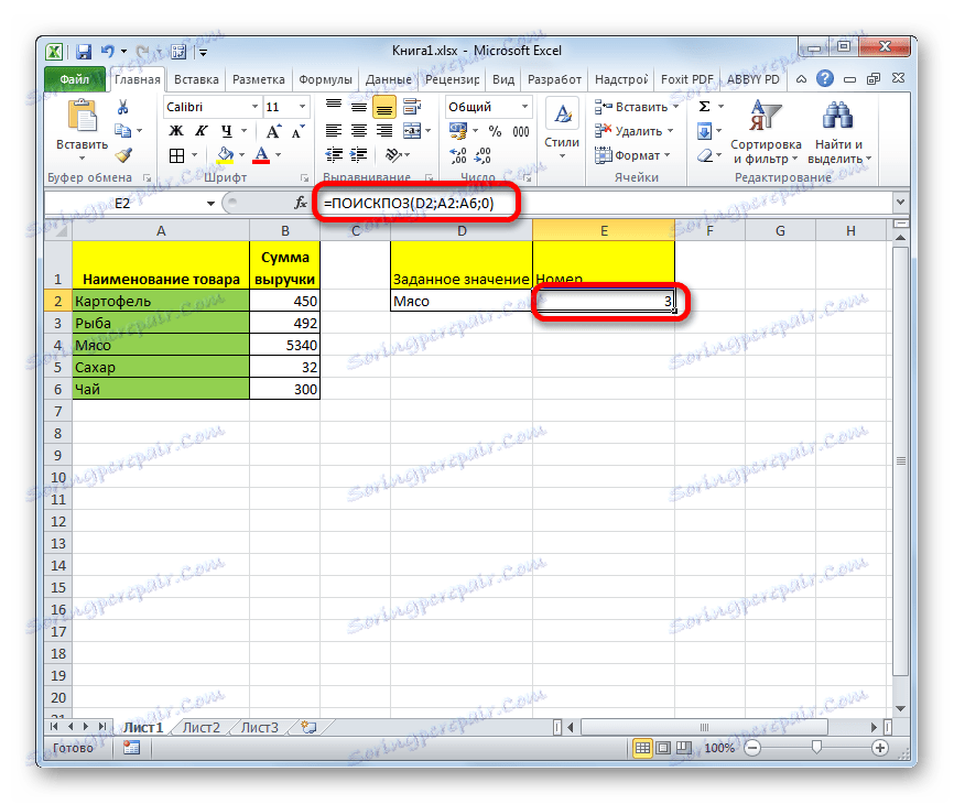
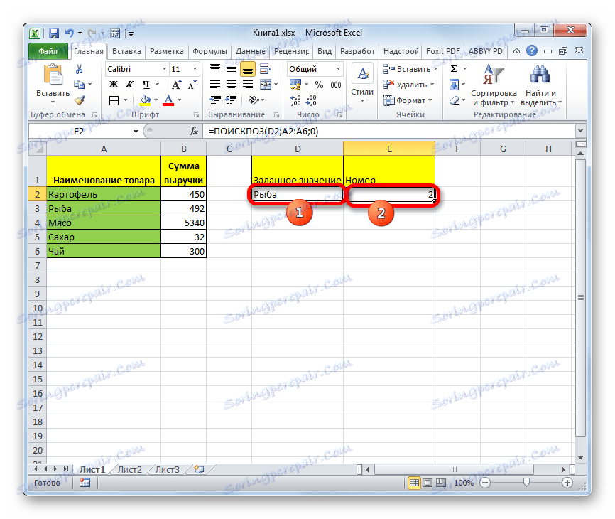
За удобство на листа добавете две допълнителни полета: "Специфична стойност" и "Номер" . В полето " Assigned стойност" караме името, което трябва да намерим. Сега нека бъде "Месо" . В полето "Номер" задайте курсора и отидете до прозореца с аргументи на оператора по същия начин, както бе обсъдено по-горе.

Способ 3: Използвайте MAP оператора за цифрови изрази

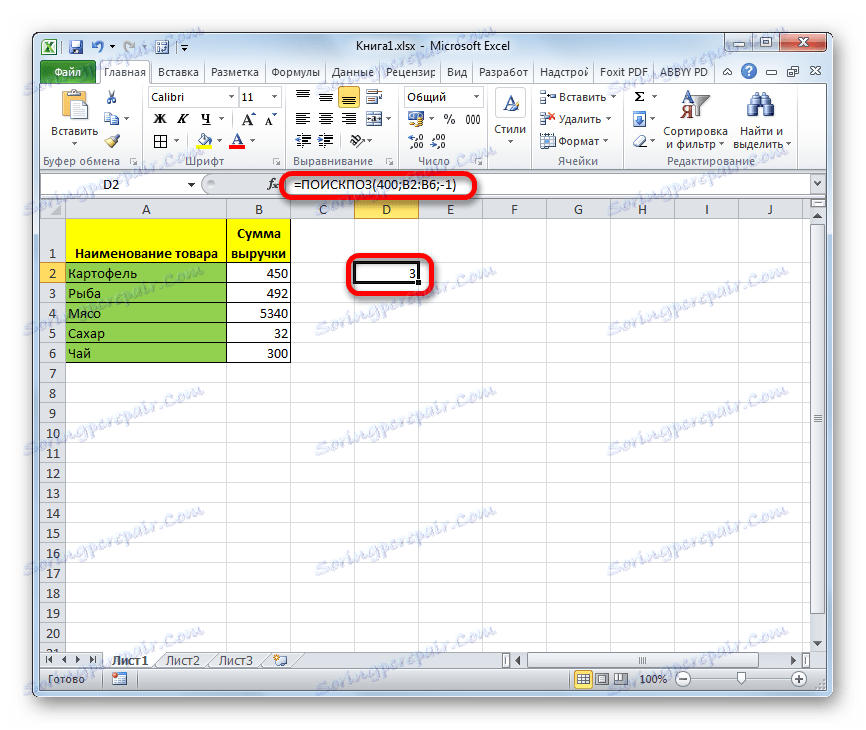
Сега нека разгледаме как сможете да използвате MATCHING, за да работите с цифрови изрази.

Задачата е да се намерят стоките за реализирането на 400 рубли либо най-близкото до тази сума във възходящ ред.

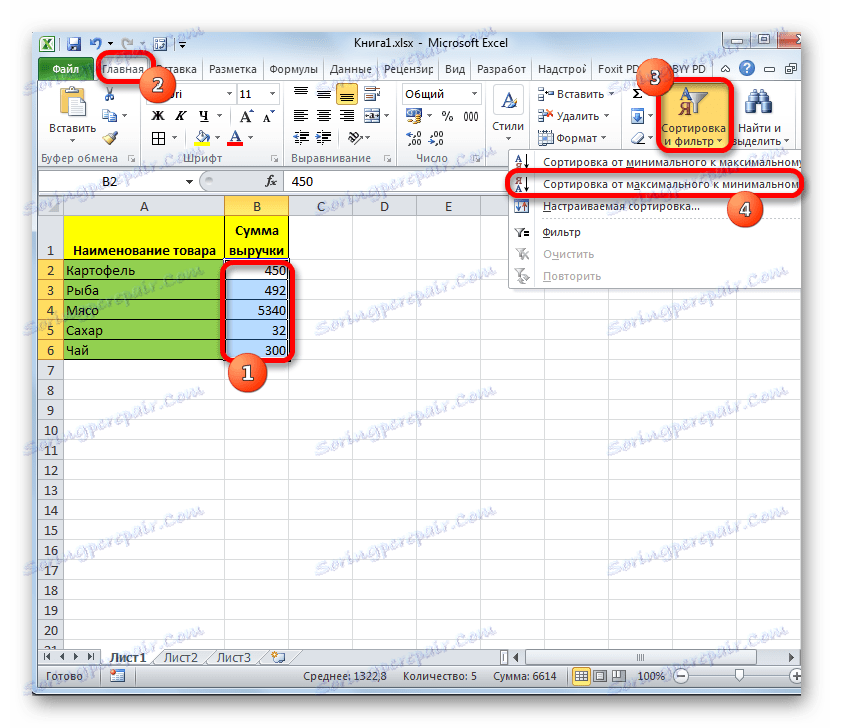
На първо място, трябва да сортираме елементите в графата "Сума" в низходящ ред. Изберете тази графа и отидете в раздела "Начало" . Кликваме върху иконата "Сортиране и филтриране" , която се намира на лентата в блока "Редактиране" . В списъка, който се показва, изберете "Сортиране от максимум до минимум" .

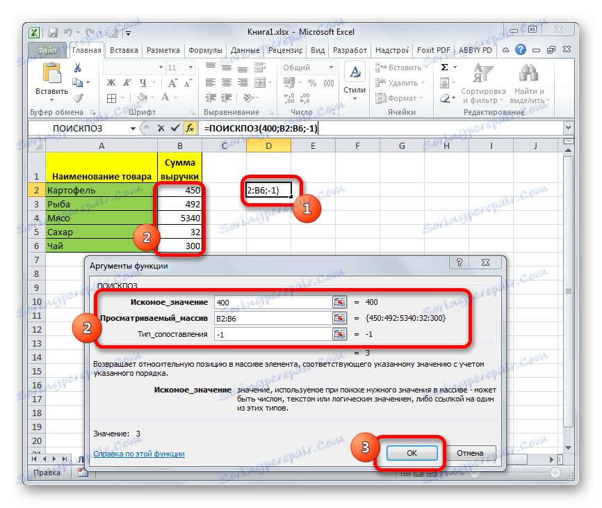
По същия начин сможете да търсите най-близката позиция до "400" в низходящ ред. Само за тази цел е нужно данните да се филтрират във възходящ ред, а в полето "Съответстващ тип" на аргументите за функциите задайте стойността на "1" .

Способ 4: Използване заедно с други оператори

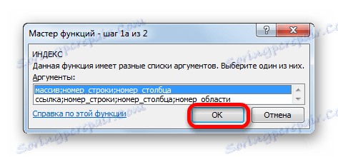
Най-ефективно е да се използва тази функция с други оператори като част от сложна формула. Най-често се използва заедно с функцията INDEX . Този аргумент извежда съдържанието на спектра, определен от номера на неговия ред либо колона, до определената клеточка. Номерацията, както в варианта на оператора POSITION , се извършва не по отношение на целия лист, а само в обхвата. Синтаксисът на тази функция е:

В този вариант, ако масивът е едноизмерен, сможете да използвате само един от двата аргумента: "Номер на ред" либо "Колонен номер" .

Особеността на връзката меж функциите INDEX и MATCH е, че последната може да се използва като първи аргумент, т.е. да се посочи позицията на ред либо колона.

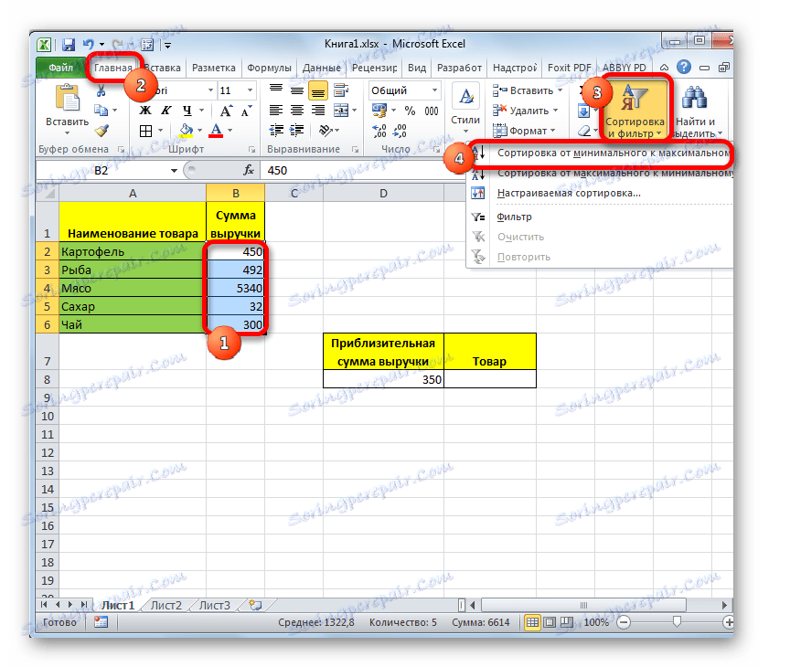
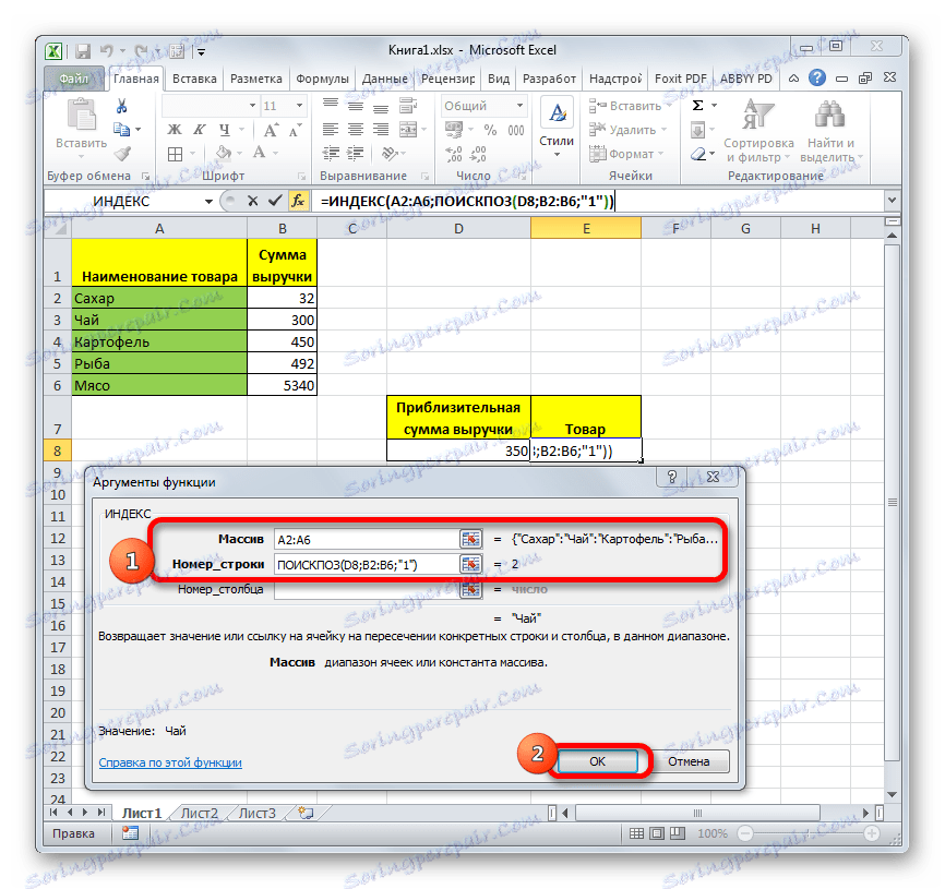
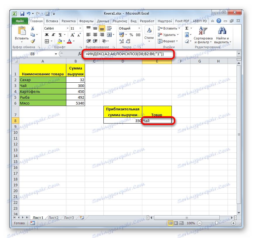
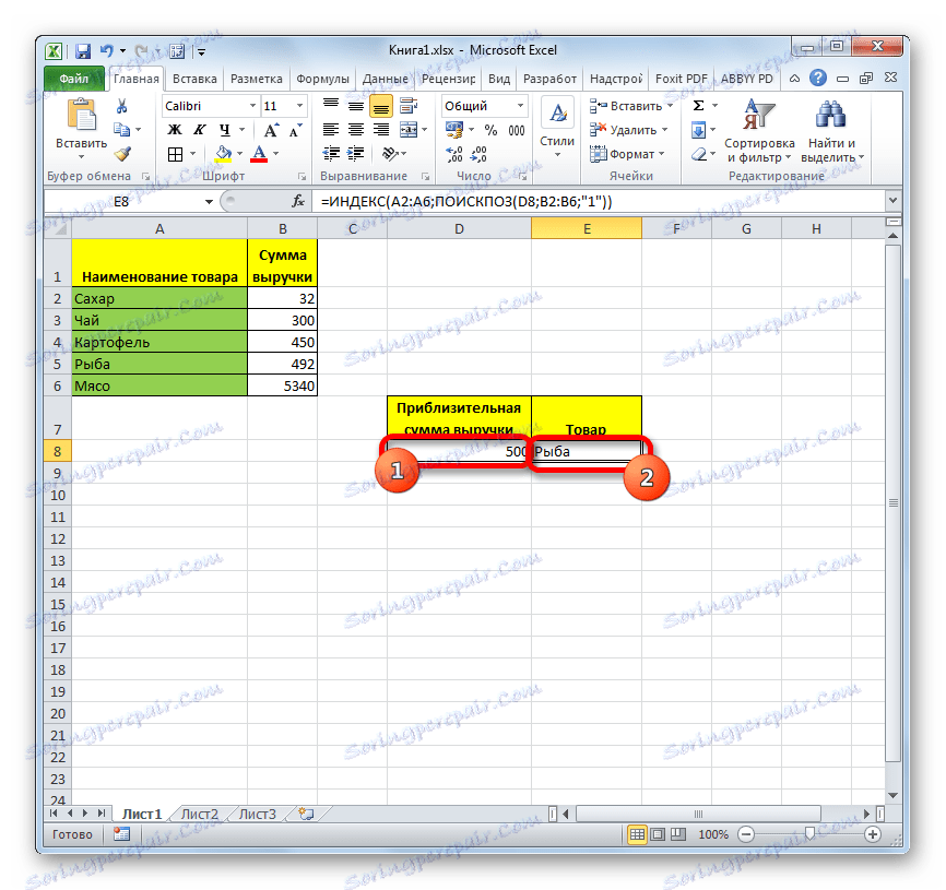
Нека да разгледаме как това може да се направи на практика, като се използва същата таблица. Ние имаме задачата да изведем името на стоките в допълнителното поле на листа "Стоки" , чийто общ размер на приходите е равен на 350 рубли либо най-близко до тази стойност в низходящ ред. Този аргумент е посочен в полето "Приблизителна сума на приходите на листа" .

Сортирайте елементите в графата "Стойност на приходите" във възходящ ред. За да направите това, изберете необходимата графа и в раздела "Начало" кликнете върху иконата "Сортиране и филтриране" и след това кликнете върху елемента "Сортиране от минимум до максимум" в менюто, показано.

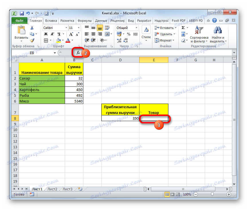
Полето "Номер на линия" ще съдържа вградената функция MATCH . Той трябва да бъде изкован ръчно, използвайки синтаксиса, споменат в самото начало на статията. Веднага напишете името на функцията — "MATCH" без кавички. След това отворете скобата. Първият аргумент на този оператор е "стойността на энтузиазма" . Той се намира на листа в полето "Приблизителна сума на приходите". Посочете координатите на клетката, съдържаща числото 350 . Поставете точка и запетая. Вторият аргумент е "Сканираният масив" . MATCHING ще разгледа обхвата, в който се намира размерът на приходите, и ще търси най-много приблизително 350 рубли. Ето защо в този вариант посочваме координатите на графата "Размер на приходите" . Отново поставяме точка и запетая. Третият аргумент е "Тип на съвпадението" . Тъй като търсим число, равно на даденото число либо най-близкото по-малко, след това зададете цифрата "1" тук . Затворете скобите.

Както сможете да видите, операторът на MAP е много комфортна функция за определяне на редовния номер на посочения елемент в масива с данни. Но ползата от него значително се увеличава, ако се използва в сложни формули.

VBA Match

Same as we have Index and Match in the worksheet as lookup functions we can also use Match functions in VBA as a lookup function, this function is a worksheet function and it is accessed by the application. worksheet method and since it is a worksheet function the arguments for Match function are similar to the worksheet function.

VBA Match Function

In this article, I will show you how to use one of the worksheet lookup function MATCH in VBA as a worksheet function.

How to Use MATCH Function in VBA Excel?

We will show you a simple example of using the Excel MATCH function in VBA.

Example #1

In VBA, we can use this MATCH formula in excel as a worksheet function. Follow the below steps to use the MATCH function in VBA.

Step 1: Create a subprocedure by giving a macro name.

Code:

Step 2: In E2 cell, we need the result, so start the code as Range (“E2”).Value =

Code:

Step 3: In E2, cell value should be the result of the MATCH formula. So in order to access the VBA MATCH function, we need to use the property “WorksheetFunction” first. In this property, we will get all the available worksheet function list.

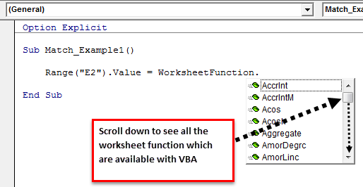
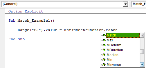
Step 4: Select the MATCH function here.

Code:

Step 5: Now, the problem starts because we don’t get the exact syntax name. Rather, we get syntax as “Arg1, Arg2, Arg3” like this. So you need to be absolutely sure of syntaxes here.

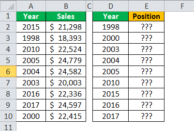
Our first argument is LOOKUP VALUE. Our LOOKUP VALUE is in the cell D2, so select the cell as Range (“D2”).Value.

Code:

Step 6: The Second argument is Table Array. Our table array range is from A2 to A10. So select the range as “Range (“A2: A10”)”

Code:

Step 7: Now, the final argument is MATCH TYPE. We need an exact match, so enter the argument value as zero.

Code:

Run the macro we will get the position of whatever the year name is there in the cell D2.

Example #2 – VBA Match From Another Sheet

Assume the same set of data from the above is there on two different sheets. For example, table array is there in the sheet name called “Data Sheet,” and Lookup Value is there in the sheet name called “Result Sheet.”

In this case, we need to refer worksheets by its name before we refer to the ranges. Below is the set of codes with sheet names.

Code:

Example #3 – VBA Match Function with Loops

Assume you have a data like this.

In these cases, it is a herculean task to write lengthy codes, so we switch to loops. Below is the set of code which will do the job for us.

Code:

This set of codes will get the result in just the blink of an eye.

Recommended Articles

This has been a guide to Excel VBA Match Function. Here we learned how to use Match Function in VBA along with some simple to advanced examples. Below are some useful excel articles related to VBA –