30 функций Excel за 30 дней: ПОИСКПОЗ (MATCH)
30 функций Excel за 30 дней: ПОИСКПОЗ (MATCH)
Вчера в марафоне 30 функций Excel за 30 дней мы находили текстовые строчки с помощью функции SEARCH (ПОИСК), также употребляли IFERROR (ЕСЛИОШИБКА) и ISNUMBER (ЕЧИСЛО) в ситуациях, когда функция выдаёт ошибку.
В 19-й денек нашего марафона мы займёмся исследованием функции MATCH (ПОИСКПОЗ). Она отыскивает значение в массиве и, если значение найдено, возвращает его позицию.
Итак, давайте обратимся к справочной инфы по функции MATCH (ПОИСКПОЗ) и разберем несколько примеров. Если у Вас есть собственные примеры либо подходы по работе с данной для нас функцией, пожалуйста, делитесь ими в комментах.
Функция 19: MATCH (ПОИСКПОЗ)
Функция MATCH (ПОИСКПОЗ) возвращает позицию значения в массиве либо ошибку #N/A (#Н/Д), если оно не найдено. Массив быть может, как сортированный, так и не сортированный. Функция MATCH (ПОИСКПОЗ) не чувствительна к регистру.
Как можно употреблять функцию MATCH (ПОИСКПОЗ)?
Функция MATCH (ПОИСКПОЗ) возвращает позицию элемента в массиве, и этот итог быть может применен иными функциями, таковыми как INDEX (ИНДЕКС) либо VLOOKUP (ВПР). К примеру:
- Отыскать положение элемента в несортированном перечне.
- Употреблять совместно с CHOOSE (ВЫБОР), чтоб перевести успеваемость учащихся в буквенную систему оценок.
- Употреблять совместно с VLOOKUP (ВПР) для гибкого выбора столбца.
- Употреблять совместно с INDEX (ИНДЕКС), чтоб отыскать наиблежайшее значение.
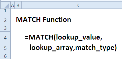
Синтаксис MATCH (ПОИСКПОЗ)
Функция MATCH (ПОИСКПОЗ) имеет последующий синтаксис:
- lookup_value (искомое_значение) – быть может текстом, числом либо логическим значением.
- lookup_array (просматриваемый_массив) – массив либо ссылка на массив (смежные ячейки в одном столбце либо в одной строке).
- match_type (тип_сопоставления) – может принимать три значения: -1, 0 либо 1. Если аргумент пропущен, это равносильно 1.
Ловушки MATCH (ПОИСКПОЗ)
Функция MATCH (ПОИСКПОЗ) возвращает положение отысканного элемента, но не его значение. Если требуется возвратить значение, используйте MATCH (ПОИСКПОЗ) совместно с функцией INDEX (ИНДЕКС).
Пример 1: Находим элемент в несортированном перечне
Для несортированного перечня можно употреблять 0 в качестве значения аргумента match_type (тип_сопоставления), чтоб выполнить поиск четкого совпадения. Если требуется отыскать четкое совпадение текстовой строчки, то в разыскиваемом значении допускается употреблять знаки подстановки.
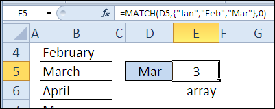
В последующем примере, чтоб отыскать положение месяца в перечне, мы можем написать заглавие месяца или полностью, или отчасти с применением знаков подстановки.
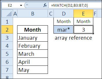
В качестве аргумента lookup_array (просматриваемый_массив) можно употреблять массив констант. В последующем примере разыскиваемый месяц введен в ячейку D5, а наименования месяцев подставлены в качестве второго аргумента функции MATCH (ПОИСКПОЗ) в виде массива констант. Если в ячейке D5 ввести наиболее поздний месяц, к примеру, Oct (октябрь), то результатом функции будет #N/A (#Н/Д).
Пример 2: Изменяем оценки учащихся c процентов на буковкы
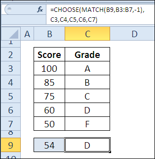
Вы сможете конвертировать оценки учащихся в буквенную систему, используя функцию MATCH (ПОИСКПОЗ) так же, как Вы делали это с VLOOKUP (ВПР). В этом примере функция применена в сочетании с CHOOSE (ВЫБОР), которая и возвращает подходящую нам оценку. Аргумент match_type (тип_сопоставления) принимаем равным -1, так как баллы в таблице отсортированы в порядке убывания.
Когда аргумент match_type (тип_сопоставления) равен -1, результатом будет меньшее значение, которое больше искомого либо эквивалентное ему. В нашем примере разыскиваемое значение равно 54. Так как такового значения нет в перечне баллов, то ворачивается элемент, соответственный значению 60. Потому что 60 стоит на четвёртом месте перечня, то результатом функции CHOOSE (ВЫБОР) будет значение, которое находится на 4-й позиции, т.е. ячейка C6, в какой находится оценка D.
Пример 3: Создаем гибкий выбор столбца для VLOOKUP (ВПР)
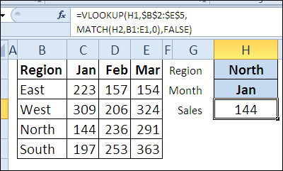
Чтоб придать больше гибкости функции VLOOKUP (ВПР), Вы сможете употреблять MATCH (ПОИСКПОЗ) для поиска номера столбца, а не агрессивно вчеркивать его значение в функцию. В последующем примере юзеры могут избрать регион в ячейке H1, это разыскиваемое значение для VLOOKUP (ВПР). Дальше, они могут избрать месяц в ячейке H2, и функция MATCH (ПОИСКПОЗ) вернет номер столбца, соответственный этому месяцу.
Пример 4: Находим наиблежайшее значение с помощью INDEX (ИНДЕКС)
Функция MATCH (ПОИСКПОЗ) непревзойденно работает в сочетании с функцией INDEX (ИНДЕКС), которую мы разглядим наиболее внимательно чуток позднее в рамках данного марафона. В этом примере функция MATCH (ПОИСКПОЗ) применена для того, чтоб отыскать из нескольких угаданных чисел наиблежайшее к правильному.
Excel MATCH Function

MATCH is an Excel function used to locate the position of a lookup value in a row, column, or table. MATCH supports approximate and exact matching, and wildcards (* ?) for partial matches. Often, MATCH is combined with the INDEX function to retrieve a value at a matched position.
- lookup_value — The value to match in lookup_array.
- lookup_array — A range of cells or an array reference.
- match_type — [optional] 1 = exact or next smallest (default), 0 = exact match, -1 = exact or next largest.
The MATCH function is used to determine the position of a value in a range or array. For example, in the screenshot above, the formula in cell E6 is configured to get the position of the value in cell D6. The MATCH function returns 5 because the lookup value («peach») is in the 5th position in the range B6:B14:
The MATCH function can perform exact and approximate matches and supports wildcards (* ?) for partial matches. There are 3 separate match modes (set by the match_type argument), as described below.
Note: the MATCH function will always returns the first match. If you need to return the last match (reverse search) see the XMATCH function. If you want to return all matches, see the FILTER function.
MATCH only supports one-dimensional arrays or ranges, either vertical and horizontal. However, you can use MATCH to locate values in a two-dimensional range or table by giving MATCH the single column (or row) that contains the lookup value. You can even use MATCH twice in a single formula to find a matching row and column at the same time.
Frequently, the MATCH function is combined with the INDEX function in order to retrieve a value at a certain (matched) position. In other words, MATCH figures out the position, and INDEX returns the value at that position. For a detailed explanation, see How to use INDEX and MATCH.
Below are simple examples of how the MATCH function can be used to return the position of values in a range. Further down the page are more advanced examples of how MATCH can be used to solve real-world problems.
Match type information
Match type is optional. If not provided, match type defaults to 1 (exact or next smallest). When match type is 1 or -1, it is sometimes referred to as «approximate match». However, keep in mind that MATCH will find an exact match with all match types, as noted in the table below:
| Match type | Behavior | Details |
|---|---|---|
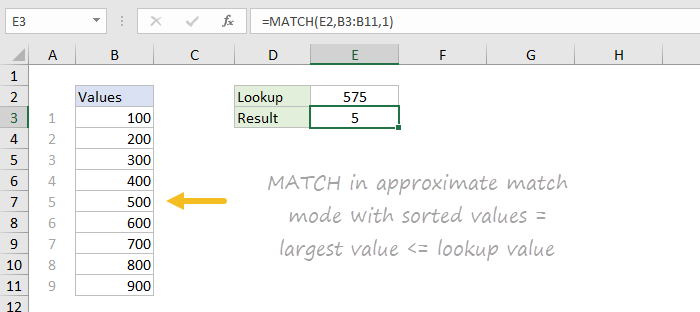
| 1 | Approximate | MATCH finds the largest value less than or equal to lookup value. Lookup array must be sorted in ascending order. |
| 0 | Exact | MATCH finds the first value equal to lookup value. Lookup array does not need to be sorted. |
| -1 | Approximate | MATCH finds the smallest value greater than or equal to lookup value. Lookup array must be sorted in descending order. |
| Approximate | When match type is omitted, it defaults to 1 with behavior as explained above. |
Caution: Be sure to set match type to zero (0) if you need an exact match. The default setting of 1 can cause MATCH to return results that «look normal» but are in fact incorrect. Explicitly providing a value for match_type, is a good reminder of what behavior is expected.
Exact match
When match type is set to zero, MATCH performs an exact match. In the example below, the formula in E3 is:

In the formula above, the lookup value comes from cell E2. If the lookup value is hardcoded into the formula, it must be enclosed in double quotes («») , since it is a text value:
Note: MATCH is not case-sensitive, so «Mars» and «mars» will both return 4.
Approximate match
When match type is set to 1, MATCH will perform an approximate match on values sorted A-Z, finding the largest value less than or equal to the lookup value. In the example shown below, the formula in E3 is:
Wildcard match
When match type is set to zero (0), MATCH can perform a match using wildcards. In the example shown below, the formula in E3 is:
This is equivalent to:

INDEX and MATCH
The MATCH function is commonly used together with the INDEX function. The resulting formula is called «INDEX and MATCH». For example, in the screen below, INDEX and MATCH are used to return the cost of a code entered in cell F4. The formula in F5 is:
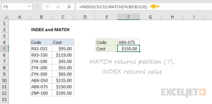
In this example, MATCH is set up to perform an exact match. The MATCH function locates the code ABX-075 and returns its position (7) directly to the INDEX function as the row number. The INDEX function then returns the 7th value from the range C5:C12 as a final result. The formula is solved like this:
See below for more examples of the MATCH function. For more details on INDEX with MATCH, see: How to use INDEX and MATCH.
Case-sensitive match
The MATCH function is not case-sensitive. However, MATCH can be configured to perform a case-sensitive match when combined with the EXACT function in a generic formula like this:
The EXACT function compares every value in array with the lookup_value in a case-sensitive manner. This formula is explained in with an INDEX and MATCH example here.
Example MATCH function for finding occurring values in Excel
MATCH function in Excel is used to find an exact match or the closest (less or more than the specified depending on the type of matching specified as an argument) value specified in the array or range of cells and returns the position number of the found element.
Examples of using the MATCH function in Excel
For example, we have a series of numbers from 1 to 10, written in cells B1:B10. Function =MATCH(3,B1,B10,0) will return the number 3, because the desired value is in cell B3, which is the third from the point of reference (cell B1).
This function is convenient for use in cases when it is necessary to return not the value contained in the desired cell, but its coordinate relative to the range in question. If arrays are used for constants, which can be represented as arrays of “key” — “value” elements, the FIND function returns a key value that is not explicitly specified.
For example, the array <"grapes"; "apple"; "pear"; "plum">contains elements that can be represented as: 1 — «grapes», 2 — «apple», 3 — «pear», 4 — «plum «, Where 1, 2, 3, 4 — the keys, and the names of fruits — values. Then the function =MATCH(«apple»,<"grapes","apple","pear","plum">,0) returns the value 2, which is the key of the second element. The counting is performed not from 0 (zero), as it is implemented in many programming languages when working with arrays, but from 1.
MATCH function is rarely used independently. It is advisable to use it in conjunction with other functions, for example, INDEX.
Formula for finding inaccurate text matches in Excel
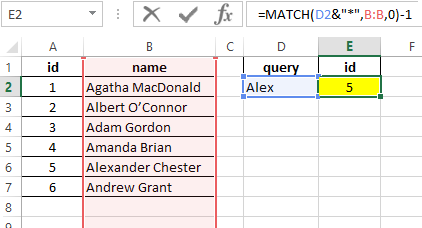
Example 1. Find the position of the first partial match of a string in a range of cells that store text values.
View source data table:
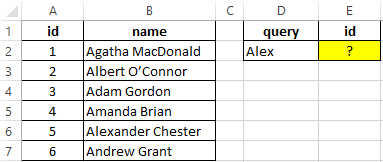
To find the position of a text string in a table, we use the following formula:
- D2 & «*» is the sought value consisting of the last name specified in cell B2 and any number of other characters (“*”);
- B:B — reference to the column B: B, in which the search is performed;
- 0 — search for exact match.
A unit is subtracted from the obtained value to match the result with the id of the entry in the table.
Comparison of two tables in Excel for the presence of discrepancies
Example 2. Excel stores two tables that appear to be the same at first glance. It was decided to compare one similar column of these tables for the presence of discrepancies. Implement a way to compare two cell ranges.
View of data table:
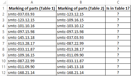
To compare the values in column B:B with the values from column A:A, use the following array formula (CTRL+SHIFT+ENTER):
MATCH function searches for a TRUE logical value in the array of logical values returned by the EXACT function (compares each element of the A2:A12 range with the value stored in cell B2 and returns an array of comparison results). If the MATCH function has found the value TRUE, the position of its first occurrence in the array will be returned. ISNA function will return FALSE if it does not accept the # N / A error value as an argument. In this case, the function IF returns the text string “is”, otherwise — “no”.
To calculate the remaining values, let us “stretch” the formula from cell C2 down to use the autocomplete function. As a result, we get:
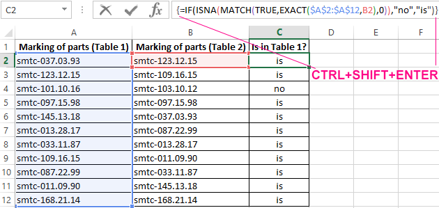
As you can see, the third elements of the lists do not match.
Finding the nearest greater knowledge in the range of Excel numbers
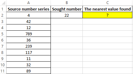
Example 3. Find the nearest smaller number to 22 in the range of numbers stored in an Excel spreadsheet column.
View source data table:
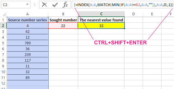
To search for the nearest larger value specified in the entire column A:A (a numerical series can be updated with new values) use the array formula (CTRL + SHIFT + ENTER):
MATCH function returns the position of the element in column A: A, which has the maximum value among the numbers that are greater than the number specified in cell B2. INDEX function returns the value stored in the found cell.
The result of the calculations:
To search for the nearest smaller value, you only need to slightly change this formula and it should also be entered as an array (CTRL + SHIFT + ENTER):