VLOOKUP Function Examples; Excel; Гугл Sheets

VLOOKUP Function Examples – Excel & Гугл Sheets

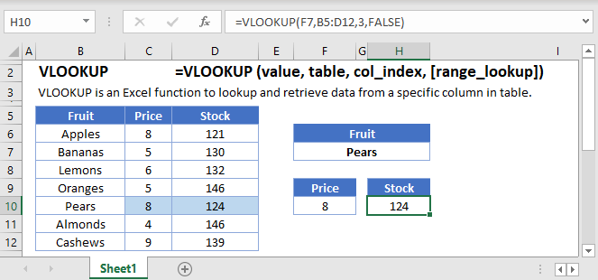
The VLOOKUP Function Vlookup stands for vertical lookup. It searches for a value in the leftmost column of a table. Then returns a value a specified number of columns to the right from the found value. It is the same as a hlookup, except it looks up values vertically instead of horizontally.

(Notice how the formula inputs appear)

VLOOKUP Function Syntax and Arguments:

lookup_value – The value you want to search for.

table_array – The data range that contains both the value you want to search for and the value you want the vlookup to return. The column containing the search values must be the left-most column.

col_index_num – The column number of the data range, from which you want to return a value from.

range_lookup – TRUE or FALSE. FALSE searches for an exact match. TRUE searches for the nearest match that is less than or equal to the lookup_value. If TRUE is chosen the left-most column (the lookup column) must be sorted ascendingly (lowest to highest).

What is the VLOOKUP function?

As one of the older functions in the world of spreadsheets, the VLOOKUP function is used to do Vertical Lookups. It has a few limitations that are often overcome with other functions, such as INDEX/MATCH. However, it does have the benefit of being a single function that can do an exact match lookup by itself. It also tends to be one of the first functions people learn about.

Basic example

Let’s look at a sample of data from a grade book. We’ll tackle several examples for extracting information for specific students.

If we want to find what class Bob is in, we would write the formula:

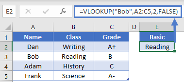
Important things to remember are that the item we’re searching for (Bob), must be in the first column of our search range (A2:C5). We’ve told the function that we want to return a value from the 2 nd column, which in this case is column B. Finally, we indicated that we want to do an exact match by placing False as the last argument. Here, the answer will be “Reading”.

Side tip: You can also use the number 0 instead of False as the final argument, as they have the same value. Some people prefer this as it’s quicker to write. Just know that both are acceptable.

Shifted Data

To add some clarification to our first example, the lookup item doesn’t have to be in column A of your spreadsheet, just the first column of your search range. Let’s use the same data set:

Now, let’s find the grade for the class of Science. Our formula would be

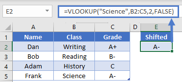
This is still a valid formula, as the first column of our search range is column B, which is where our search term of “Science” will be found. We’re returning a value from the 2 nd column of the search range, which in this case is column C. The answer then is “A-“.

Wildcard usage

The VLOOKUP function supports the use of the wildcards “*” an “?” when doing searches. For instance, let’s say that we’d forgotten how to spell Frank’s name, and just wanted to search for a name that starts with “F”. We could write the formula

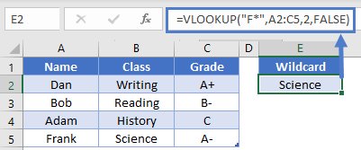
This would be able to find the name Frank in row 5, and then return the value from 2 nd relative column. In this case, the answer will be “Science”.

Non-exact match

Most of the time, you’ll want to make sure that the last argument in VLOOKUP is False (or 0) so that you get an exact match. However, there are a few times when you might be searching for a non-exact match. If you have a list of sorted data, you can also use VLOOKUP to return the result for the item that is either the same, or next smallest. This is often used when dealing with increasing ranges of numbers, such as in a tax table or commission bonuses.

Let’s say that you want to find the tax rate for an income entered cell D2. The formula in D4 can be:

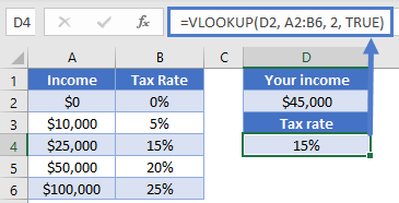
The difference in this formula is that our last argument is “True”. In our specific example, we can see that when our individual inputs an income of $45,000 they will have a tax rate of 15%.

Note: Although we usually are wanting an exact match with False as the argument, it you forget to specify the 4 th argument in a VLOOKUP, the default is True. This can cause you to get some unexpected results, especially when dealing with text values.

Dynamic column

VLOOKUP requires you to give an argument saying which column you want to return a value from, but the occasion may arise when you don’t know where the column will be, or you want to allow your user to change which column to return from. In these cases, it can be helpful to use the MATCH function to determine the column number.

Let’s consider our grade book example again, with some inputs in E2 and E4. To get the column number, we could write a formula of

This will try to find the exact position of “Grade” within the range A1:C1. The answer will be 3. Knowing this, we can plug it into a VLOOKUP function and write a formula in E6 like so:

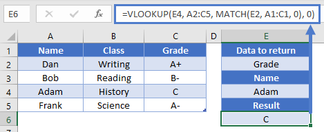
So, the MATCH function will evaluate to 3, and that tells the VLOOKUP to return a result from the 3 rd column in the A2:C5 range. Overall, we then get our desired result of “C”. Our formula is dynamic now in that we can change either the column to look at or the name to search for.

VLOOKUP limitations

As mentioned at the beginning of the article, the biggest downfall of VLOOKUP is that it requires the search term to be found in the left most column of the search range. While there are some fancy tricks you can do to overcome this <link to CHOOSE article>, the common alternative is to use INDEX and MATCH. That combo gives you more flexibility, and it can sometimes even be a faster calculation.

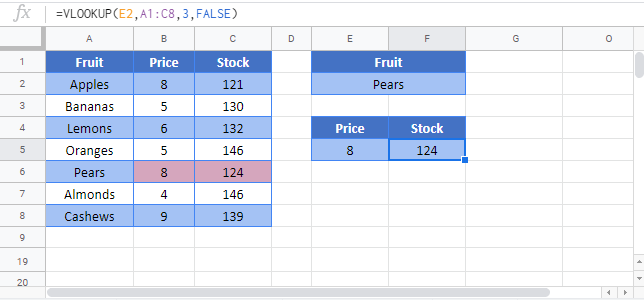
VLOOKUP in Гугл Sheets

The VLOOKUP Function works exactly the same in Гугл Sheets as in Excel:

Additional Notes

Use the VLOOKUP Function to perform a VERTICAL lookup. The VLOOKUP searches for an exact match (range_lookup = FALSE) or the closest match that is equal to or less than the lookup_value (range_lookup = TRUE, numeric values only) in the first row of the table_array. It then returns a corresponding value, n number of rows below the match.

When using an VLOOKUP to find an exact match, first you define an identifying value that you want to search for as the lookup_value. This identifying value might be a SSN, employee ID, name, or some other unique identifier.

Next you define the range (called the table_array) that contains the identifiers in the top row and whatever values that you ultimately wish to search for in the rows below it. IMPORTANT: The unique identifiers must be in the top row. If they are not, you must either move the row to the top, or use MATCH / INDEX instead of the VLOOKUP.

Third, define row number (row_index) of the table_array that you wish to return. Keep in mind that the first row, containing the unique identifiers is row 1. The second row is row 2, etc.

Last, you must indicate whether to search for an exact match (FALSE) or nearest match (TRUE) in the range_lookup. If the exact match option is selected, and an exact match is not found, an error is returned (#N/A). To have the formula return blank or “not found”, or any other value instead of the error value (#N/A) use the IFERROR Function with the VLOOKUP.

To use the VLOOKUP Function to return an approximate match set: range_lookup = TRUE. This option is only available for numeric values. The values must be sorted in ascending order.

VLOOKUP Examples in VBA

You can also use the VLOOKUP function in VBA. Type:
application.worksheetfunction.vlookup(lookup_value,table_array,col_index_num,range_lookup)
For the function arguments (lookup_value, etc.), you can either enter them directly into the function, or define variables to use instead.

Excel Practice Worksheet

Practice Excel functions and formulas with our 100% free practice worksheets!

Excel VLOOKUP Formula Examples – Including how to create dynamic vlookup formulas

Excel VLOOKUP Formula Examples – Including how to create dynamic vlookup formulas

In part 1 of this series we took a look at VLOOKUP formula basics. If you want to learn how a VLOOKUP formula works, or know someone else who is struggling with VLOOKUPs, check out the first article “Discover a simple way to understand how VLOOKUP formulas work in Excel“, and come back to this article.

Here in part 2, we have a 14 minute video that explains three different ways to write the VLOOKUP formula for exact matches. If you have never used the COLUMNS function or MATCH function with VLOOKUP, you are in for a treat because you will find out how to turn the standard VLOOKUP into a dynamic formula. As usual I have included a sample workbook with a table of fictional employee data for you to download and follow along with the examples.

Download the VLOOKUP Employee Table Sample Workbook

In order to follow along with the video and article please download the Sample Workbook “VLOOKUP_Employee_Table.xlsx” by clicking here

Note: the sample workbook has been tested on Excel 2010 (32-bit, English language version) and you may get different results in other version of Excel. If you find that you can’t use this workbook on your version of Excel, please let us know using the comment section below.

The sample download workbook contains slightly different cell references compared to the workbook used in the video, but the data itself is identical and provides a convenient way for you to practise your VLOOKUP formulas.

VLOOKUP Tutorial Video Part 2

Watch our 14 minute video to help you understand three different ways of writing the VLOOKUP formula for exact matches. Click on the video below to play it and listen to my audio commentary.

Video Transcript

Note: The video was transcribed by SpeechPad.com and then edited into the form you see below.

We’re going to have a look at three different ways to write VLOOKUP formulas. One is a straightforward, simple approach, the second is using the columns function, and the third is using the MATCH function.

Here we have an employee LOOKUP table with the employee ID on the left. You see we’ve got employee full name, SSN, department, start date, and earnings for each of these employees.

Employee Lookup Table – see sample download spreadsheet. If you haven’t yet downloaded a copy of the spreadsheet, head back up and get it now so you can follow along.

Change the drop-down selection from EMP003 to EMP002 and watch the formula output update

Note about the Data

None of the names here are real people, they’re all computer-generated names. So if you see someone’s name that you recognize, it isn’t that person.

Learn more about Data Validation

By the way, if you want to learn more about data validation, you should check out my book “Power Tips for Excel.” That takes you through some data validation tips and tricks.

What we will cover in this video

Now I’m going to take you through three different ways of writing the VLOOKUP formula.

1. Simple way – type in numbers for column index number
2. COLUMN function – use the COLUMN function to specify column index number
3. MATCH function – use the MATCH function to specify column index number

The first is the standard approach, the second uses the COLUMN function, and the third uses the MATCH function. While the first way is the simple way, it is actually not the most efficient in this case. We’ll go through method one, then we’ll check out the column method and the match method which in my opinion are usually more useful.

VLOOKUP Method One – Type in numbers for column index number (not dynamic)

The simple method is to use the VLOOKUP formula without any other functions. Go to cell C5 and we will set up the VLOOKUP to pull up “Full Name” using the employee ID. In the formula bar, type =VLOOKUP, then type out the full VLOOKUP formula. When I click on E5 I also press the F4 key (three times) to lock this to absolute references so it doesn’t move from column B ($B5).

Press the F4 key to change cell reference style to absolute column reference ($B5 where $ means column B stays fixed or “absolute”)

It is usually a good idea to exclude column headings when you specify the data range for “table_array” in your VLOOKUP formulas

Complete the VLOOKUP formula by specifying 2 for “col_index_num” and FALSE for “range_lookup” type, meaning 2nd column in table_array and FALSE to return an exact match.

Now, you see it’s just put the full name in each of these boxes, which we don’t want.

This is what happens after copying the formula right. Excel does not know that you want to look up different values, so it looks up the same value from column 2 in every cell.

We need to change the formula in each cell to update the col_index_num. Each cell now has the correct VLOOKUP column offset, and returns the correct lookup value.

VLOOKUP Method Two – Use the COLUMN function to specify column index number (semi-dynamic)

Method two uses the columns function, which you can see here. So the formula is going to end up like this, it’s going to be a VLOOKUP with the standard parameters. But it’s also going to use the function COLUMNS with an array, and I explain that later, with a FALSE at the end for an exact match.

Method 2 – VLOOKUP with the COLUMN function

For the table_array, I will select the data excluding the column headings (as before, this is good practice when writing VLOOKUP formulas). Press Control + Shift + Right arrow, Control + Shift + Down arrow, and that will select all the data in the table (this works because there are no empty data cells). Press the F4 key to lock that to absolute references.

And now, for the column index number, for “Full Name”, I want it to come out with a 2. And what the function COLUMNS does is it counts the number of columns in a particular array, where an array is just a group of cells on the worksheet.

We want the array to start at B9 and go up to C9. I’m going to lock the range reference to the column B, by inserting a dollar sign ($B9:C9). And so when I copy this across, you’ll that the first cell in the range reference stays in column B while the second cell in the range reference moves from column C to column D to column E etc. depending on how far I copy across (e.g. $B9:E9)

Specify the array used inside the COLUMNS function as $B:C9

So for employee EMP004 it has found “Denton Q Dale”. And now I’m going to copy the VLOOKUP formula, using Control + Alt + V to copy and paste special formulas only, so I don’t overwrite the existing cell formats.

When the VLOOKUP formula is copied across, the COLUMNS($B9:C9) function dynamically takes care of the col_index_num so there is no need to manually update it for every cell.

So in cell G5, the COLUMNS function looks at the range $B9 to G9, and counts how many columns are there. So that would be one column, two columns, three columns, four columns, five columns, six columns, and when it counts six columns, it will give the VLOOKUP formula, the right parameter for column index number.

VLOOKUP Method Three – Use the MATCH function to specify column index number (Dynamic)

Method three uses the MATCH function instead of the columns function to give you the column index number. The MATCH function returns the relative position of an item in an array that matches a specified value.

So for example, if I want to find out where “Full Name” was in this array, what I do is type “=MATCH(“. First function argument is lookup_value so I select C4 (“Full Name”. The second function argument is lookup_array so I select B9:G9 (the data table headings). The third and last function argument is match_type and we want an exact match so type 0 or FALSE.

We build up the VLOOKUP + MATCH formula in steps. The first step is to write the MATCH function and check that it works correctly.

I will modify the MATCH formula to make the range B9:G9 into absolute references by selecting it and pressing F4. The reason is that we want to copy this across and have it update with the correct range, so copy the formula using CONTROL + C, then paste it to the cells on the right, pressing CONTROL + ALT + V to paste special as formulas.

When the formula is copied across to the right, you can see the results are 2, 3, 4, 5 and 6. What it’s done is evaluates the correct column number to use in our lookup formula by matching the contents of row 4 to the contents of row 9.

You can see that copying across the MATCH formula results in the right column number being calculated.

Time to combine the MATCH function and VLOOKUP function

Now we now work through the VLOOKUP formula to see why the MATCH function can be very useful.

This is the combined VLOOKUP + MATCH formula: “=VLOOKUP($B$5, $B$10:$G$59, MATCH(C$4, $B$9:$G$9, 0), FALSE)”

For the third function argument column_index, we use the MATCH function to lookup up the value “Full Name” in cell C4, and find its position in the range of column headings in B9:G9.

Note the use of absolute references to lock the first argument of MATCH lookup_value to row 4, and lock the second argument of MATCH lookup_array to B9:G9. Set the match_type to 0 for exact match.

Copy the VLOOKUP + MATCH formula from cell C5 using the keyboard combination CONTROL + C, then paste special as formulas into cells D5:G5 using the keyboard combination CONTROL + ALT + V for the paste special dialog box.

This is the result:

We have completed the VLOOKUP + MATCH formula and copied it across to all cells in our lookup table. Note that if you change the values in row 4, the VLOOKUP formulas in row 5 dynamically update to lookup up the correct column.

What could go wrong with Dynamic VLOOKUPs?

Here’s a brief list of things that could go wrong with your dynamic VLOOKUP formulas. It’s by no means a comprehensive list, but covers a few fundamental errors:

• Using COLUMNS function (Method 2) when the order of your lookup table headers does not match the order of your data table headers (e.g. “Full Name, SSN, Department, Start Date” vs. “Full Name, Department, SSN, Start Date”)
• When using the MATCH function (Method 3) your lookup table headers do not match your data table headers (e.g. misspelling “Depatment” instead of “Department”)
• Your absolute references might not be correct, and as you copy your dynamic VLOOKUP formula into other cells the COLUMNS() or MATCH() function could be looking up the wrong cells.

Time for you to practise your VLOOKUP formulas

If you haven’t already downloaded the sample workbook, you can do so by clicking here.

Learn How to Combine IF Function with VLOOKUP

VLOOKUP is a powerful function to perform lookup in Excel. It performs a row-wise lookup until a match is found. The IF function performs a logical test and returns one value for a TRUE result, and another for a FALSE result. IF and VLOOKUP functions are used together in multiple cases: to compare VLOOKUP results, to handle errors, to lookup based on two values. To use the IF and VLOOKUP functions together you should nest the VLOOKUP function inside the IF function.

Combine IF Function with VLOOKUP

You can use IF and VLOOKUP together nesting the VLOOKUP function inside the IF function. The following will present a more detailed overview of the uses of IF function with VLOOKUP.

Comparing values to VLOOKUP result

IF and VLOOKUP are used together mostly to compare the results of VLOOKUP to another value. In the following example, based on the list in cells A1:B6, to find out if the name mentioned in cell D2 has a bonus which is based on sales over $2,500:

• Select cell E2 by clicking on it.
• Assign the formula =IF(VLOOKUP(D2,A2:B6,2,FALSE)>2500,»Yes»,»No») to cell E2.
• Press Enter to apply the formula in cell E2.

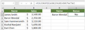
This will return the result No as Baron Wendal had sales of $2,350. You can also compare VLOOKUP results to cell values in a similar way. All you need to do is to set the cell reference as the condition inside the IF function.

Handling errors

Another common use of IF function with VLOOKUP is to handle errors. In the previous example, assign the value Jason Williams to cell D2. To find the sales, assign the formula = VLOOKUP(D2,A2:B6,2,FALSE) to cell E2.

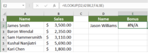
This will return a #N/A error. The name Jason Williams does not exist in cells A2:A6. To handle this error with your own custom message, you will nest the VLOOKUP and ISNA functions inside an IF function. To do that:

• Select cell E2 by clicking on it.
• Assign the formula = IF(ISNA(VLOOKUP(D2,A2:B6,2,FALSE)),»Name not found»,VLOOKUP(D2,A2:B6,2,FALSE)) to cell E2.
• Press enter to apply the formula to cell E2.

This will return Name not found. The ISNA function checks if the result of the VLOOKUP is a #N/A error, and executes the corresponding IF condition. You can set other text messages or even a 0 or blank ( “” ) as the output.

Lookup Based on two values

You can also use IF and VLOOKUP together to perform a lookup based on two values. In this example, cells A1:C6 contains the price for products in two different shops. To find the price of the product in cell E2:

• Select cell G2 by clicking on it.
• Assign the formula =IF(F2=»Shop 1″,VLOOKUP(E2,A2:C6,2,FALSE),VLOOKUP(E2,A2:C6,3,FALSE)) to cell G2.
• Apply the formula to G2 by pressing Enter.

This will return $3.50. The IF function checks if the value in cell F2 is Shop 1 or 2. According to this condition, the VLOOKUP then returns the corresponding price for the product.

Excel has several very effective functions when it comes to lookup values in other columns. One of these functions is VLOOKUP. It is a very powerful lookup and reference function for looking up data. Combined with the IF function, VLOOKUP can perform more advanced lookups that help to analyze data more effectively.

Still need some help with Excel formatting or have other questions about Excel? Connect with a live Excel expert here for some 1 on 1 help. Your first session is always free.

Are you still looking for help with the IF function? View our comprehensive round-up of IF function tutorials here.