Excel Minus Formula

In excel we do not have any inbuilt formula for subtraction or minus, we use minus operator (-) to do the arithmetical subtraction in excel, to subtract two values from each other we need to also use the equals to operator to make minus a formula, for example, = value 1- value 2 is a minus formula where we subtract value 1 from value 2, note that the values should be in the same format to avoid error in formula.

How to Use Minus Formula in Excel?

Assume we have 5 in cell A1 and 3 in cell B1. I want to subtract the value in B1 from A1. I want the result to be shown in cell C1. The formula in the cell C1 should read like this =A1 – B1.

We can also directly enter the values to the cell C1 itself.

Even though we can directly enter the numbers to the formula, it is always recommended to give cell references. Because giving cell references makes the formula dynamic and updates the value automatically if there are any changes.

Examples of Minus Calculation

Example #1

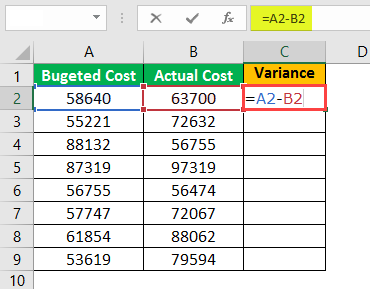
I have data on Budgeted Cost vs. Actual Cost for the year 2018. The finance department supplied me with these two data. I need to find out the variance amount whether the budgeted cost is within the limit or not?

How do I find out the variance amount? I need to deduct the budgeted cost from the actual cost.

I need to deduct B2 from A2 using the minus formula.

Example 1.1.1

From the above result, it is clear that only one item is within the budget, i.e., C6 cell. If the variance is negative, then it is over the budgeted number, and if the variance is positive, then it is within the budgeted number.

Интересно почитать: Как создать таблицу в excel пошаговая инструкция с формулами

Example #2

We know the basics of minus calculation. In this example, we will look at how to deal with one negative number and one positive number.

I have data on Quarterly profit and loss numbers.

I need to find the variance from Q1 to Q2, Q3 to Q4, Q5 to Q6.

The usual formula should be Variance = Q1 – Q2, Variance = Q3 – Q4, Variance = Q5 – Q6.

Case 1:

Now look at the first variance in the Q1 loss was -150000 in the second Q2 profit is 300000, and the overall variance should be a profit of 150000. But formula displays -450000. This is one of the drawbacks of blindly using the minus formula in excel.

We need to alter the formula here. Rather than subtracting Q1 from Q2, we need to add Q1 to Q2. Since there are a positive number and negative numbers, we need to include the plus sing here. The basic of mathematics is plus * minus = minus.

Case 2:

Now look at the third variance in the Q5 loss was -75000 and in Q6 loss was -125000. The variance should be -50000, not +50000.

In this way, we need to do the subtraction operations in excel. You should know the basics of mathematics to deal with these kinds of situations.

Example #3

Below is the data are given to me by the sales manager. This data is the individual sales data for his team. Data includes individual target and individual actual sales contribution.

He asked me to find out the variance and efficiency level percentage for each employee.

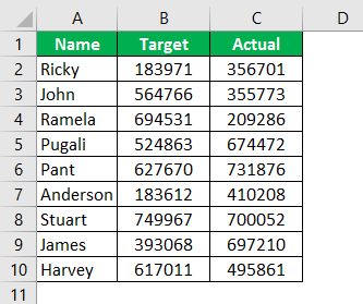
Here first things I need to find the variance, and the formula is Actual – Target, for efficiency, the formula is Actual / Target, and for Variance %, the formula is Efficiency % – 1.

Интересно почитать: Проценты в эксель формула

Calculate Variance Amount

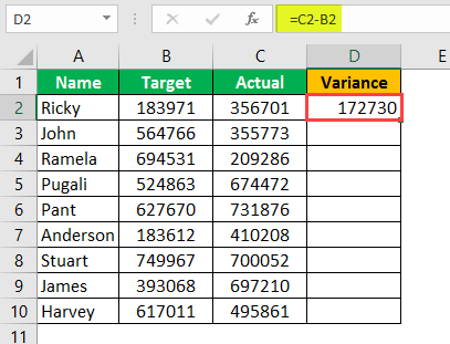
The variance amount is calculated by subtracting Actual from the Target number.

Now drag the formula to cell D10 for the other values to be determined,

Calculate Efficiency Percentage

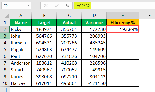
Efficiency is calculated by dividing the Actual by Target. (if the result shows in decimals, apply percentage formatting)

Now drag the formula to cell E10 for the other values to be determined,

Calculate Variance Percentage

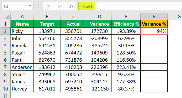
Variance percentage is calculated by deducting 1 from an efficiency percentage.

Now drag the formula to cell F10 for the other values to be determined,

Things to Remember

Apply percentage formatting in case of decimal results.
We can either directly enter the numbers or give cell referenceGive Cell ReferenceCell reference in excel is referring the other cells to a cell to use its values or properties. For instance, if we have data in cell A2 and want to use that in cell A1, use =A2 in cell A1, and this will copy the A2 value in A1.read more .
Giving cell reference makes the formula dynamic.
Always keep in mind the basic mathematics rules.
Try to learn the BODMAS rule in mathematics.

Excel works!

Что будет, если из 12-00 отнять 21-00 в Excel? По идее, если время — это число, то обязано получиться отрицательное число. Но, как показано на картинке, будет ворачиваться значение = огромному количеству символов ##### (диез, сетка либо хеш). Как создать, чтоб отрицательное время в Excel отображалось прекрасно и корректно? Как применять отрицательное время в следующих вычислениях формулами?

Интересно почитать: Как в excel изменить формулу

1 метод. Отрицательное время в Excel. Убрать копированием

Просто скопируйте значение с обилием #, как значение в другую ячейку. Можно применять специальную вставку.

Либо измените формат на числовой. Как это создать, можно прочесть в данной для нас статье.

2 метод. Обыкновенные формулы

Просто помножьте отрицательное время на -1. Либо добавьте еще функцию =ЕСЛИ(), как показано на картинке ниже

Если значение ячейки <0, то значение * -1

Так же можно в условии поменять местами наименьшее и большее время.

3 метод. Поменять формат отображения времени

Вначале, Excel употребляет систему дат, начинающуюся с 1 января 1900 года. Можно переключиться на систему использования 1904. Зайдите Файл — Характеристики — Характеристики Excel — Добавочно — раздел «При пересчете данной для нас книжки» — Употреблять систему дат 1904.

Отрицательные значения времени будут отображаться верно. К огорчению, этот метод может ввести ваших коллег в недоумение, так как на другом компе без включения галочки этот файл будут смотреться снова же ошибочно. Если готовы всем разъяснять, то этот метод вам 🙂

Не забудьте снять галочку опосля проведения операций, ведь сейчас таковая система дат всераспространена на все ваши книжки Excel!

4 метод. Функция ТЕКСТ

Функцию =ТЕКСТ тоже комфортно применять в таковых вариантах. К примеру:

где функция ABS возвращает модуль числа (т.е. его положительное значение). А функция ТЕКСТ уже конвертирует число в подходящий формат « -ч:мм:сс» . Эта формула хороша тем, что можно вернуть конкретно отрицательное значение в формате времени.

Но это не самое наилучшее решение, т.к. применять его в следующих формулах не получится (формула будет считать данные в ячейке текстом). Для верного отображения идеальнее всего переводить значение в число (1ый метод).